Hypothesis Testing

Lecture 21

While you wait…

• Go to your ae project in RStudio.

• Make sure all of your changes up to this point are committed and pushed, i.e., there’s nothing left in your Git pane.

• Click Pull to get today’s application exercise file: ae-17-hypothesis-testing.qmd.

• Wait till the you’re prompted to work on the application exercise during class before editing the file.

Recap: sampling uncertainty

What if this was my dataset?

# A tibble: 2 × 2
  term        estimate
  <chr>          <dbl>
1 (Intercept)    2.56 
2 log_inc        0.718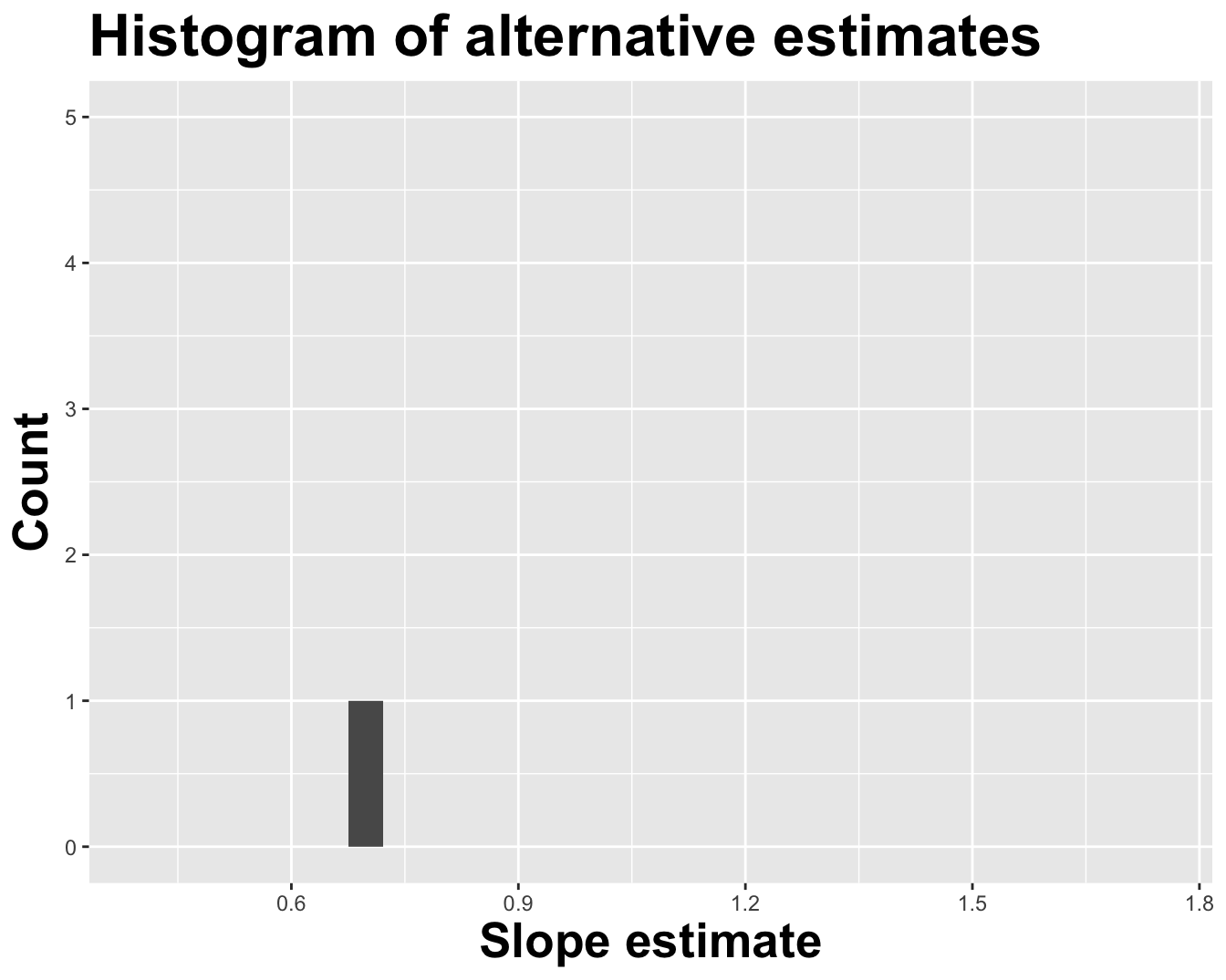

What if this was my dataset instead?

# A tibble: 2 × 2
  term        estimate
  <chr>          <dbl>
1 (Intercept)   -0.250
2 log_inc        0.964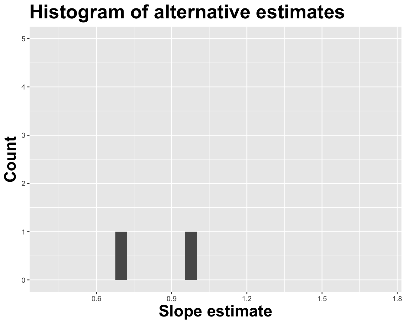

What if this was my dataset instead?

# A tibble: 2 × 2
  term        estimate
  <chr>          <dbl>
1 (Intercept)    0.468
2 log_inc        0.885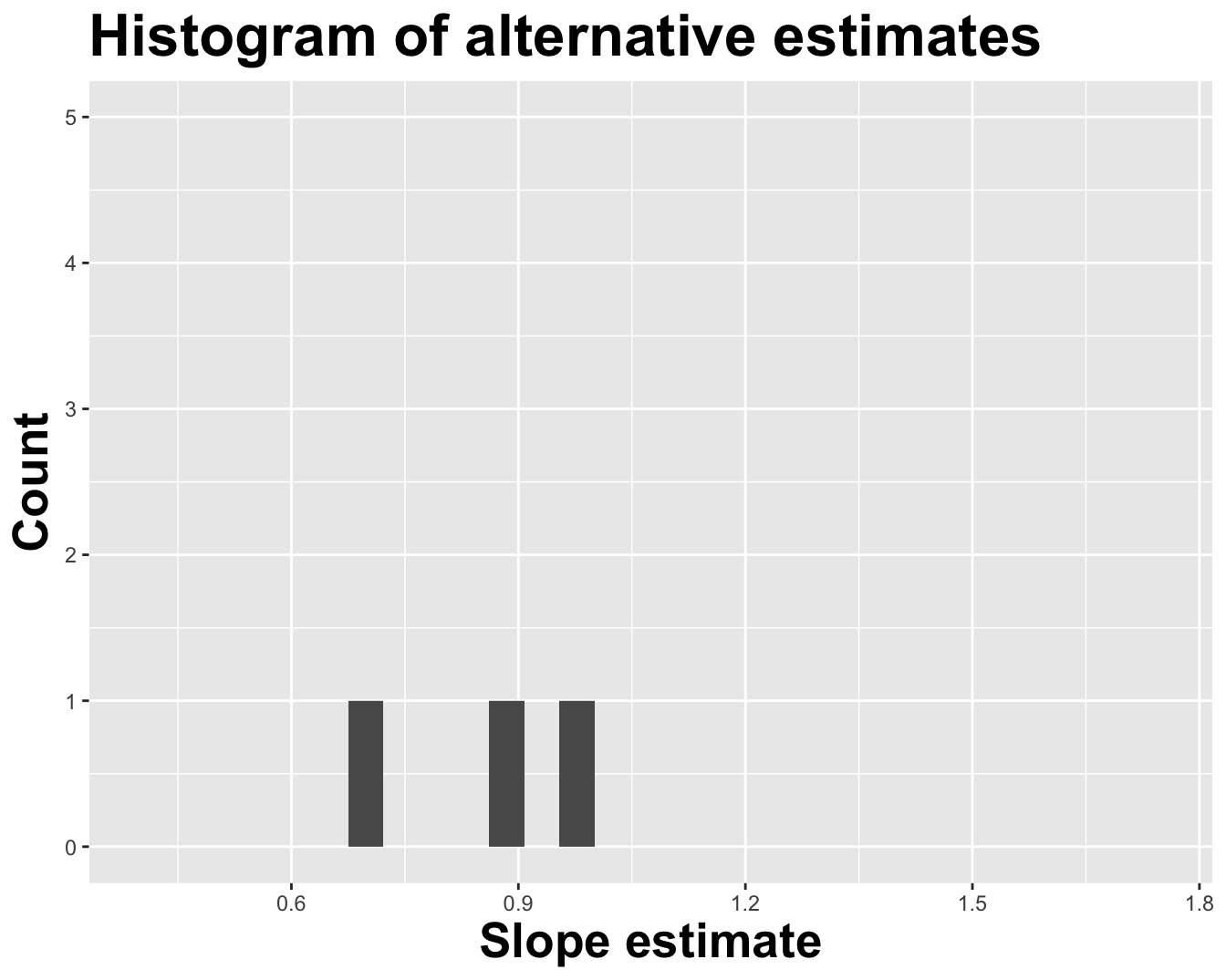

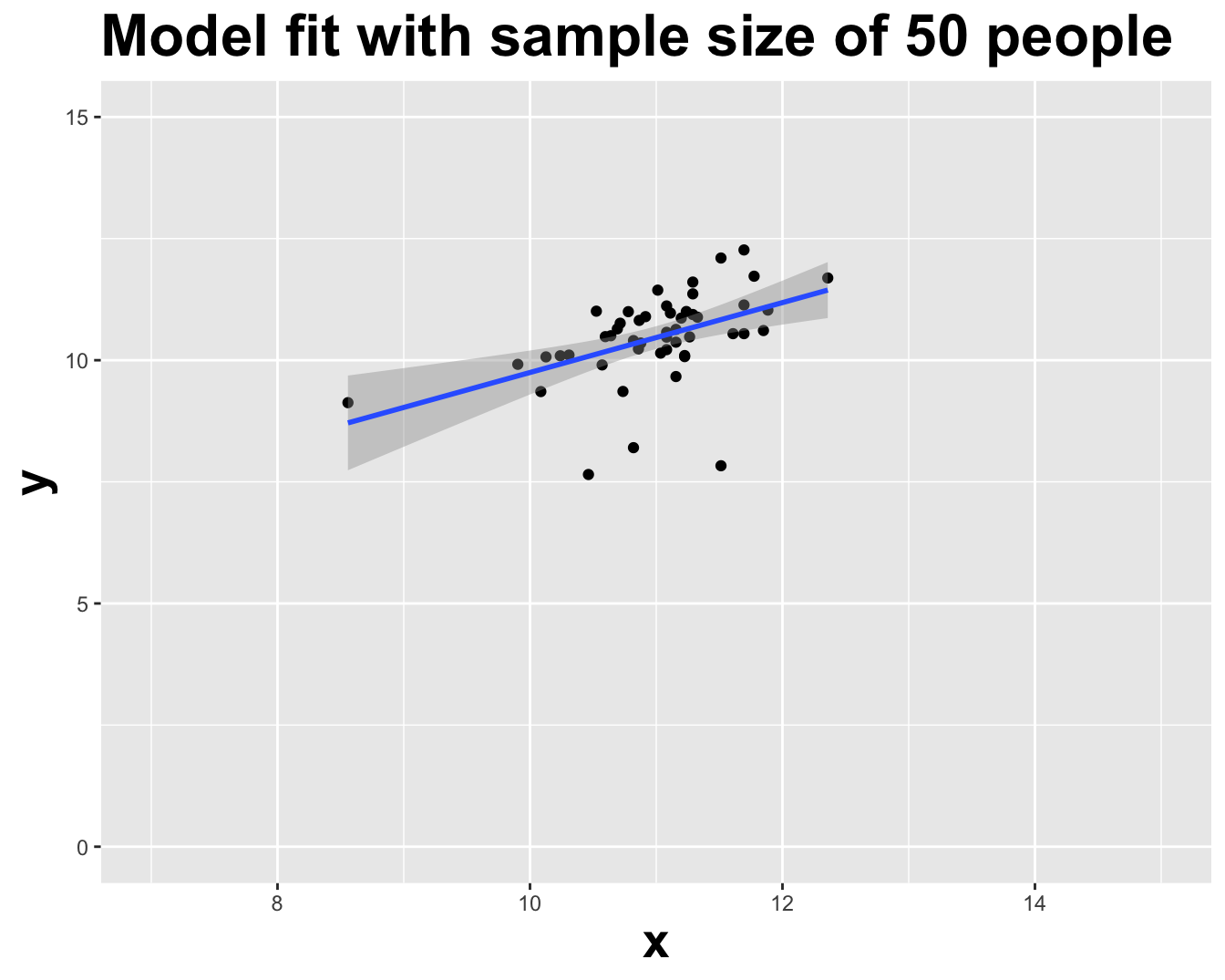
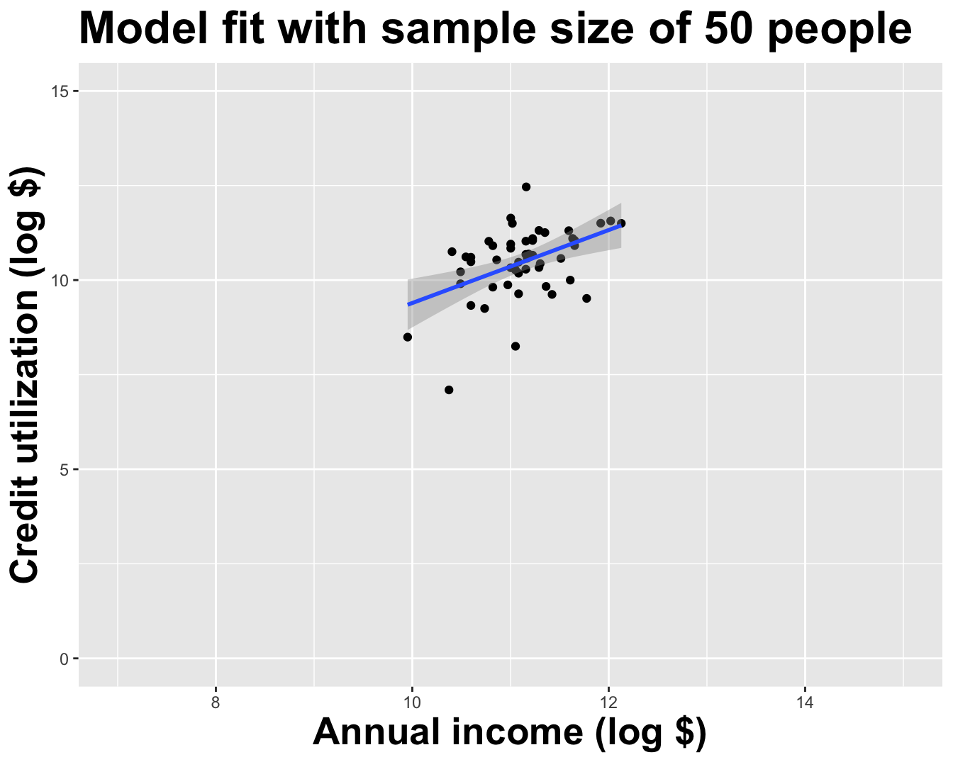
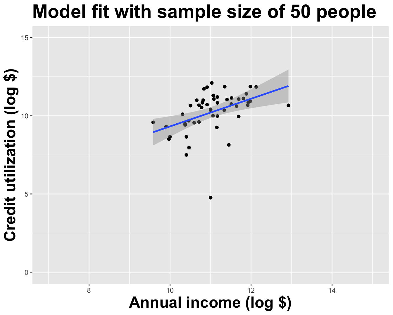
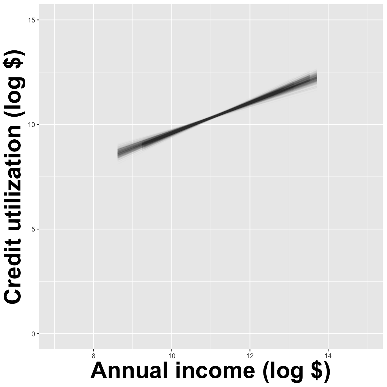
Rinse and repeat 1000 times…

Sampling uncertainty

How sensitive are the estimates to the data they are based on?

. . .

• Very? Then uncertainty is high, results are unreliable;
• Not very? Uncertainty is low, results are more reliable.

That was for n = 50. What if I was starting with n = 1000?

Sampling uncertainty decreased!

Bootstrapping

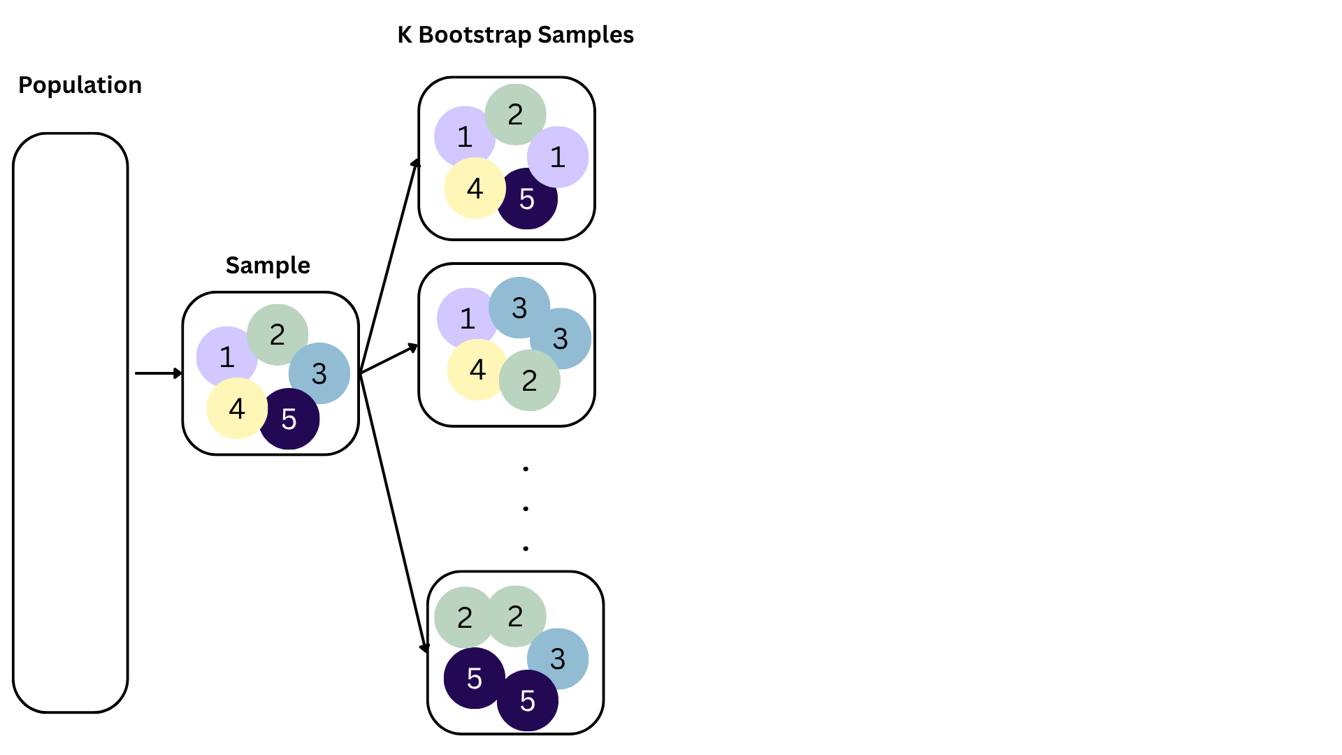
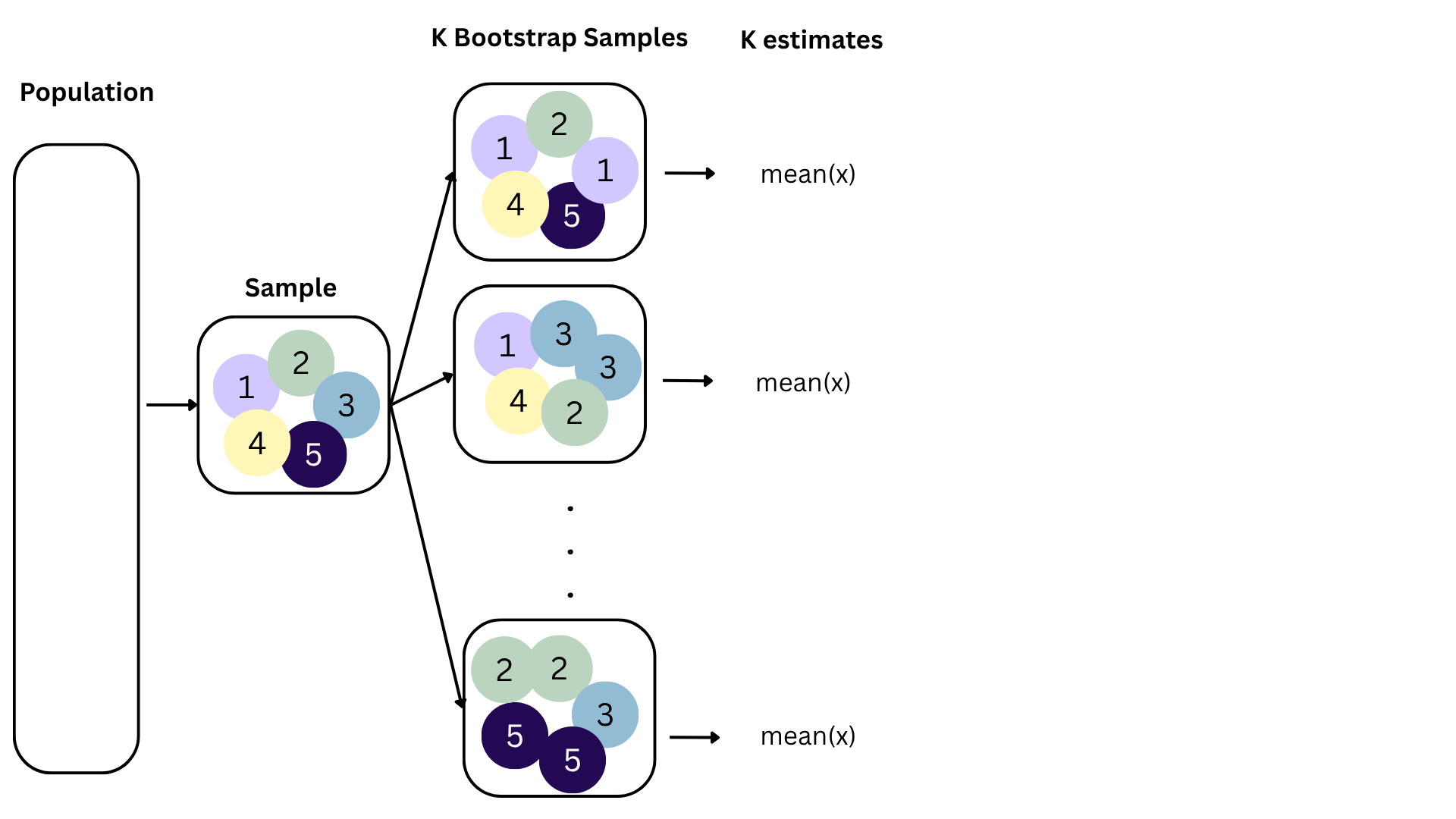
• Data collection is costly, so we have to do our best with what we already have;

• We approximate this idea of “alternative, hypothetical datasets I could have observed” by resampling our data with replacement;

• We construct a new dataset of the same size by randomly picking rows out of the original one:

  • Some rows will be duplicated;
  • Some rows will not appear at all;
  • The new dataset is different from the original;
  • Different dataset >> different estimate

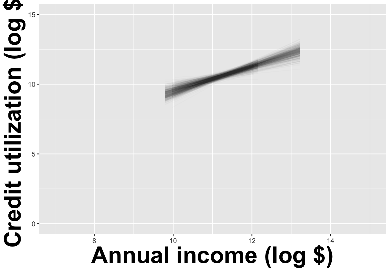
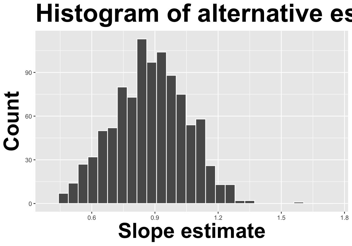
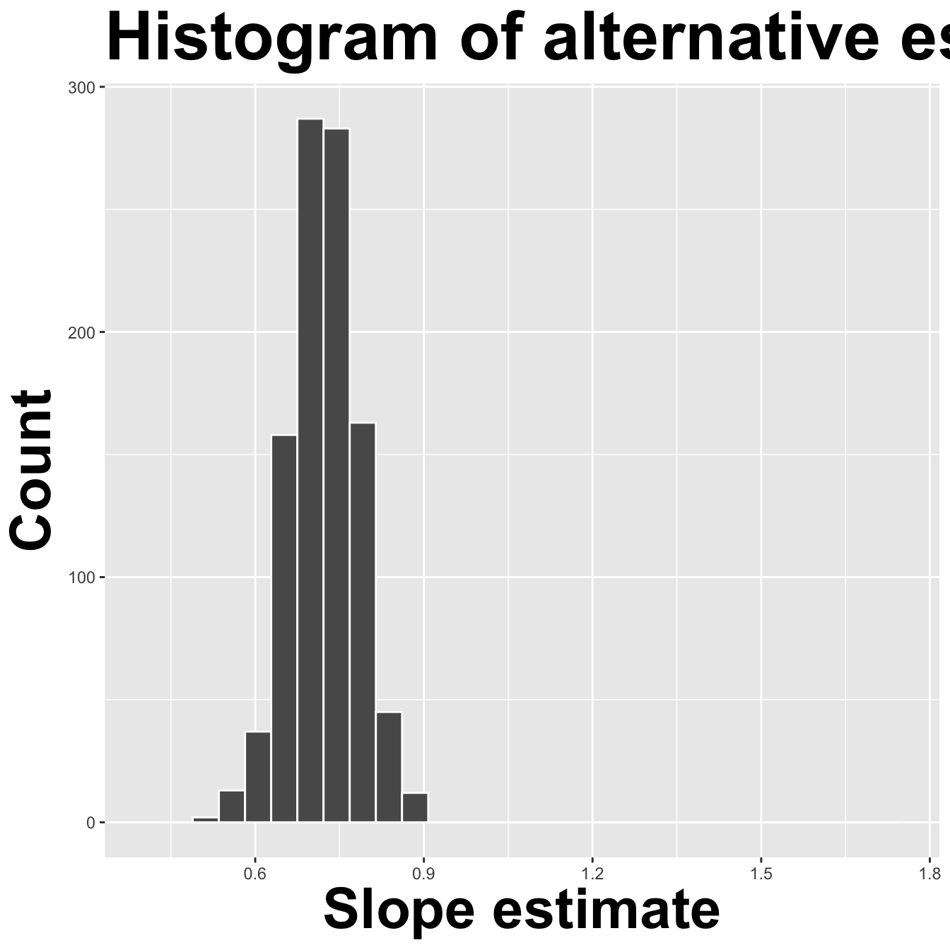
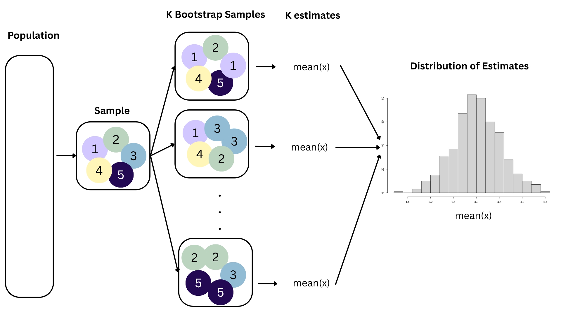
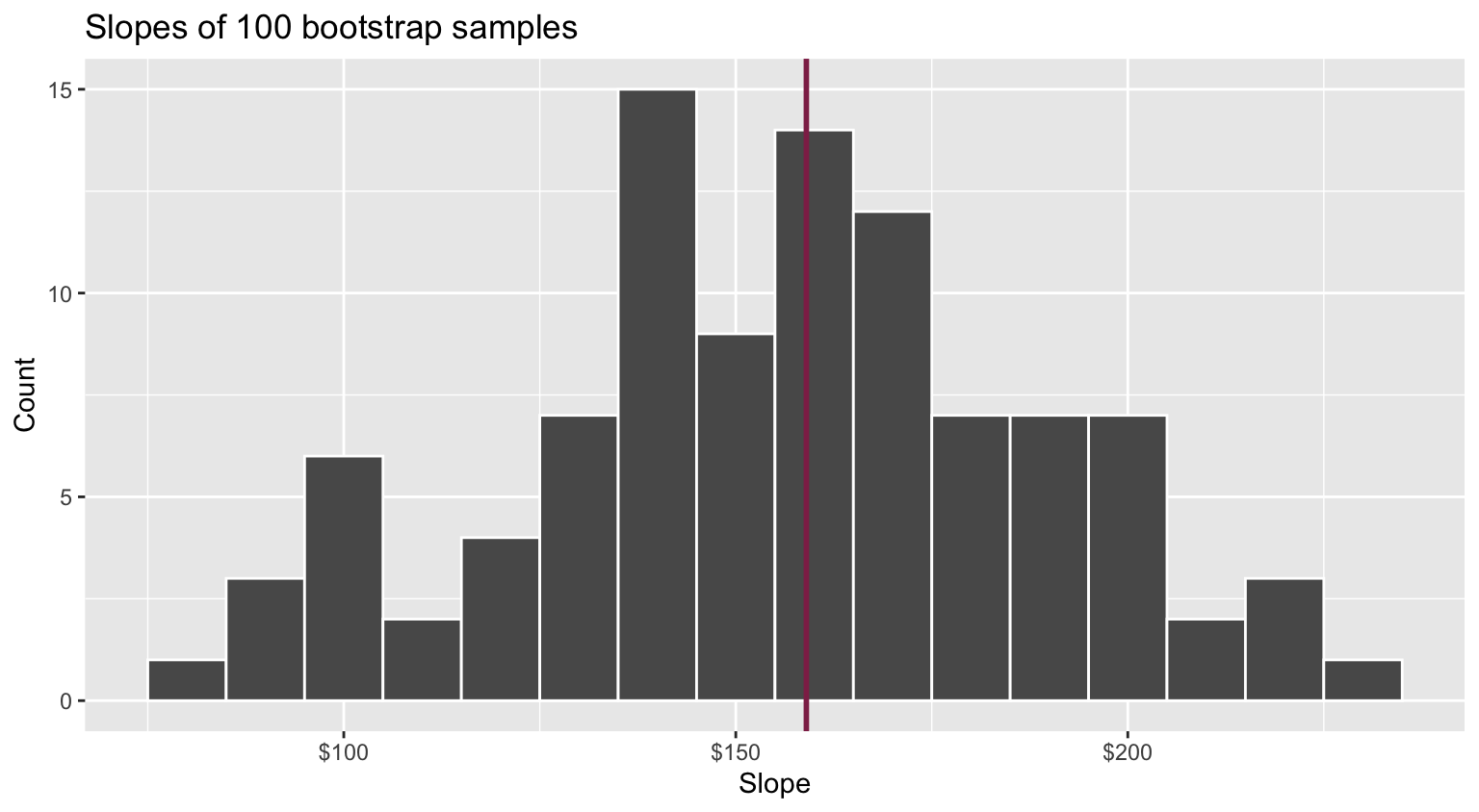
• Repeat this processes hundred or thousands of times, and observe how the estimates vary as you refit the model on alternative datasets.

• This gives you a sense of the sampling variability of your estimates.

Bootstrapping Procedure

Bootstrapping

Bootstrapping

Bootstrapping

Bootstrapping

Bootstrapping

Bootstrapping

Confidence intervals

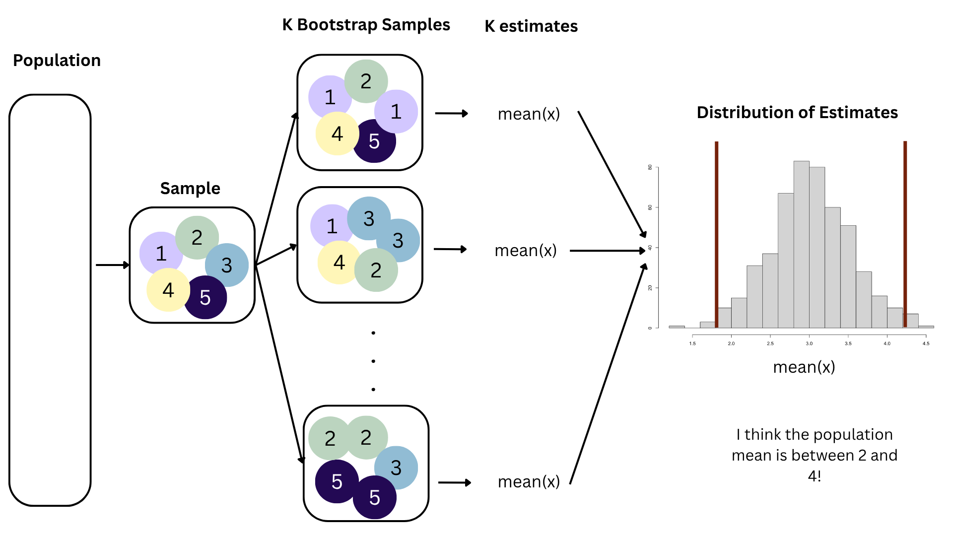
• Point estimation: report your single number best guess for the unknown quantity;

• Interval estimation: report a range, or interval, or values where you think the unknown quantity is likely to live;

  • Interval should be wide enough to capture the truth with high probability;
  • Interval should be narrow enough to be informative;

• Unfortunately, there is a trade-off. You adjust the confidence level to try to negotiate the trade-off;

• Common choices: 90%, 95%, 99%.

Precision vs. accuracy

Recap: Computing Confidence Interval

Friday’s Data: Houses in Duke Forest

• Data on houses that were sold in the Duke Forest neighborhood of Durham, NC around November 2020
• Scraped from Zillow
• Source: openintro::duke_forest

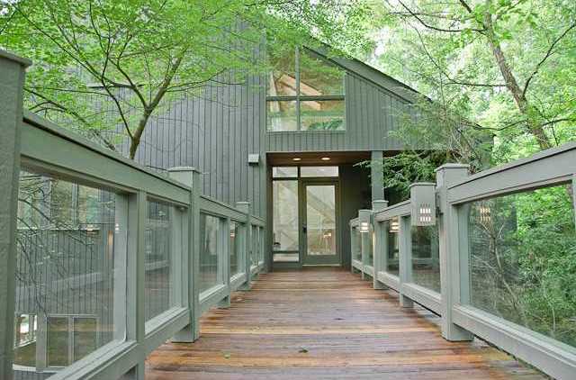
Goal: Use the area (in square feet) to understand variability in the price of houses in Duke Forest.

Point Estimate

observed_fit <- duke_forest |>
  specify(price ~ area) |>
  fit()

observed_fit

# A tibble: 2 × 2
  term      estimate
  <chr>        <dbl>
1 intercept  116652.
2 area          159.

Slopes of bootstrap samples

Fill in the blank: For each additional square foot, the model predicts the sale price of Duke Forest houses to be higher, on average, by between ___ and ___ dollars.

Slopes of bootstrap samples

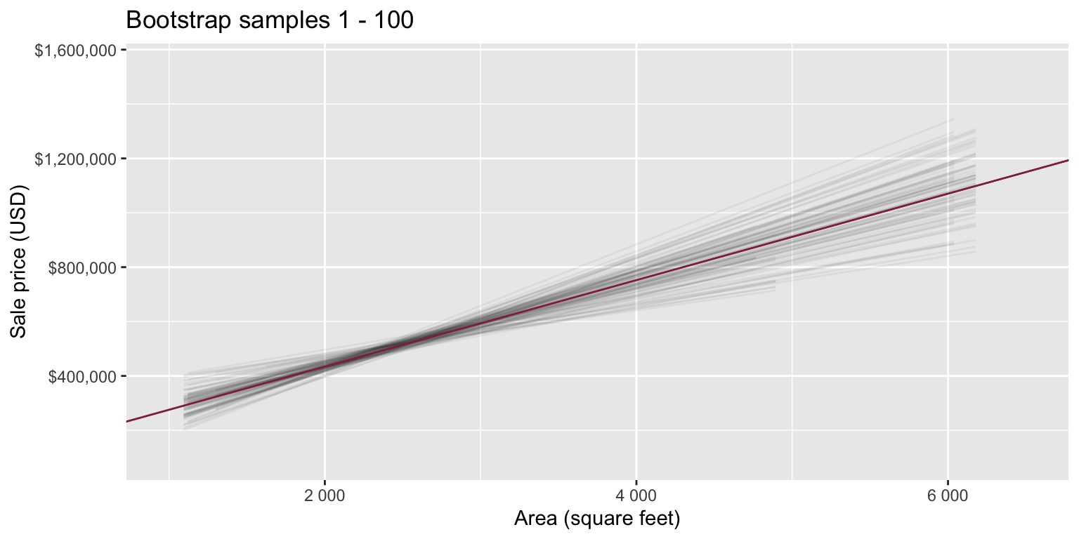
Fill in the blank: For each additional square foot, we expect the sale price of Duke Forest houses to be higher, on average, by between ___ and ___ dollars.

95% confidence interval

• A 95% confidence interval is bounded by the middle 95% of the bootstrap distribution
• We are 95% confident that for each additional square foot, the model predicts the sale price of Duke Forest houses to be higher, on average, by $90.17 to $215.39.

Where do the bounds come from?

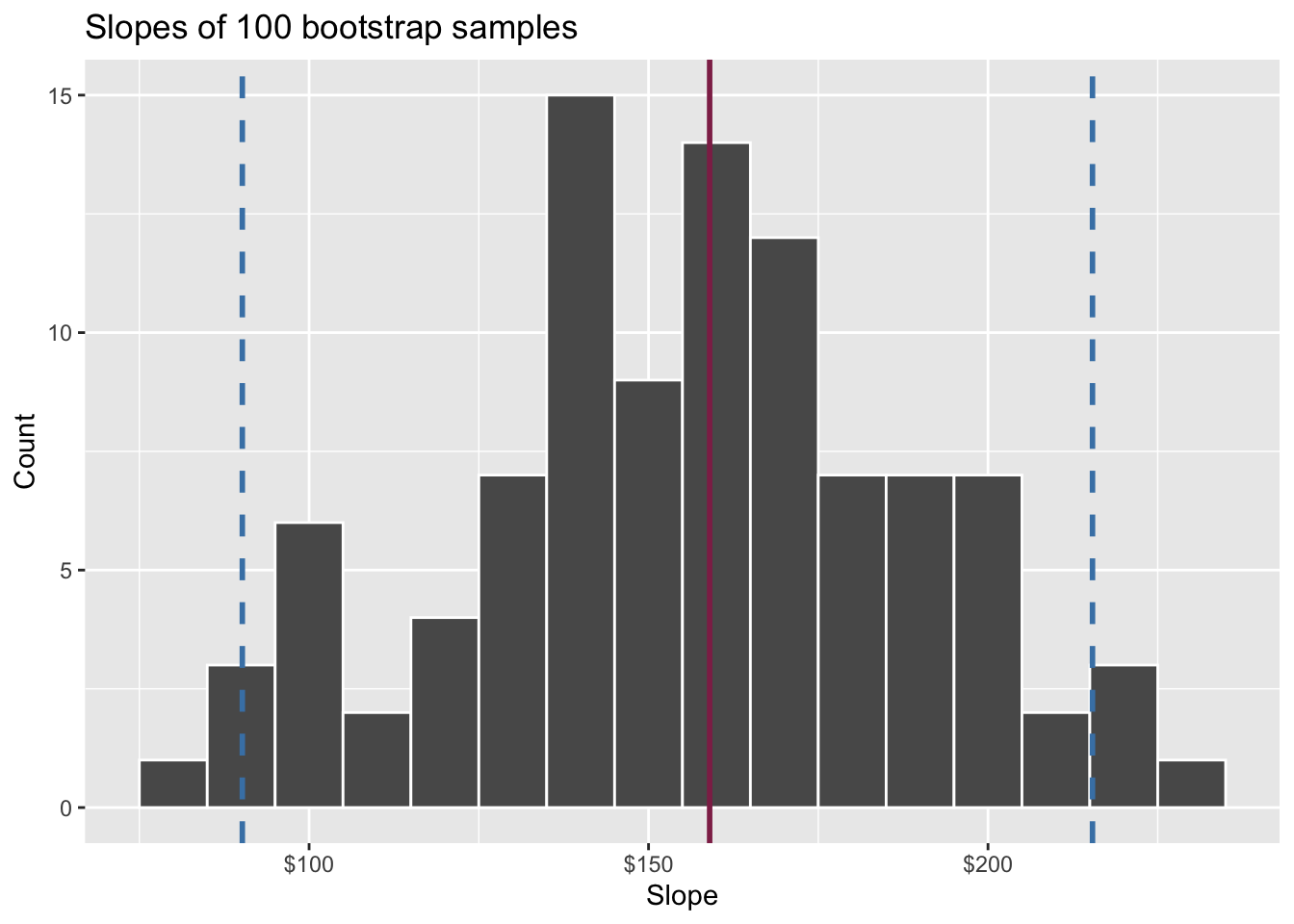
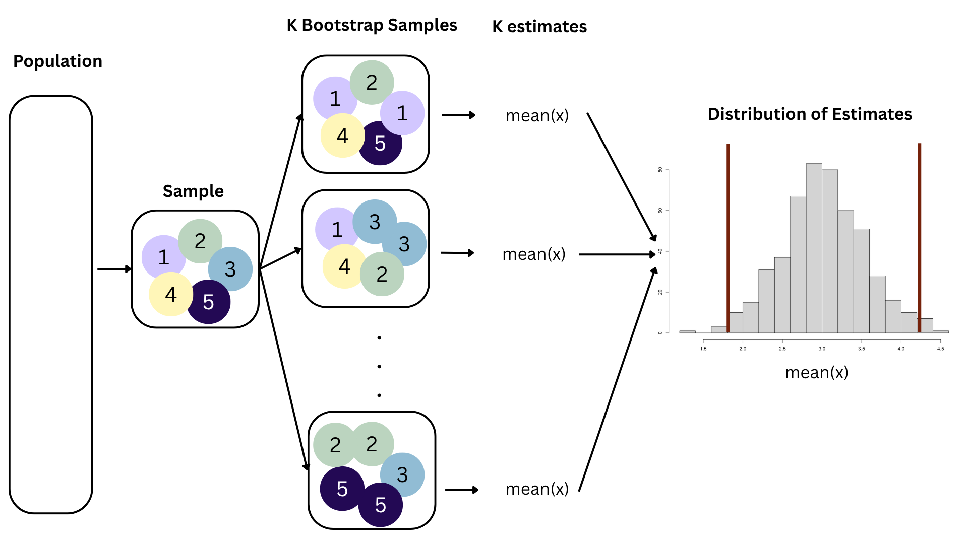
• Think IQR! 50% of the bootstrap distribution is between the 25% quantile on the left and the 75% quantile on the right. But we want more than 50%

• 90% of the bootstrap distribution is between the 5% quantile on the left and the 95% quantile on the right;

• 95% of the bootstrap distribution is between the 2.5% quantile on the left and the 97.5% quantile on the right;

• And so on.

Recap (again!!)

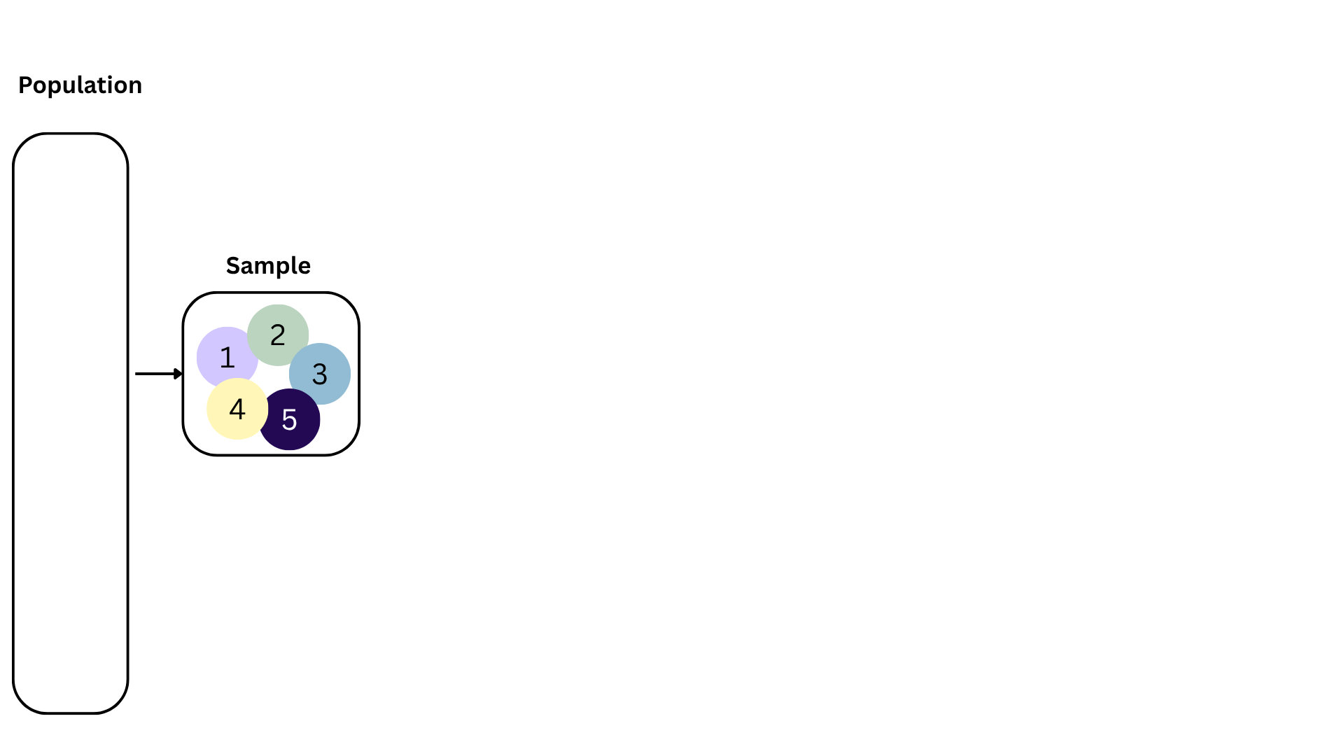
• Population: Complete set of observations of whatever we are studying, e.g., people, tweets, photographs, etc. (population size = \(N\))

• Sample: Subset of the population, ideally random and representative (sample size = \(n\))

• Sample statistic \(\ne\) population parameter, but if the sample is good, it can be a good estimate

• Statistical inference: Discipline that concerns itself with the development of procedures, methods, and theorems that allow us to extract meaning and information from data that has been generated by stochastic (random) process

• We report the estimate with a confidence interval, and the width of this interval depends on the variability of sample statistics from different samples from the population

• Since we can’t continue sampling from the population, we bootstrap from the one sample we have to estimate sampling variability

Hypothesis testing

Hypothesis testing

A hypothesis test is a statistical technique used to evaluate competing claims using data

• Null hypothesis, \(H_0\): An assumption about the population. “There is nothing going on.”

• Alternative hypothesis, \(H_A\): A research question about the population. “There is something going on”.

. . .

Note: Hypotheses are always at the population level!

Setting hypotheses

• Null hypothesis, \(H_0\): “There is nothing going on.” The slope of the model for predicting the prices of houses in Duke Forest from their areas is 0, \(\beta_1 = 0\).

• Alternative hypothesis, \(H_A\): “There is something going on”. The slope of the model for predicting the prices of houses in Duke Forest from their areas is different than, \(\beta_1 \ne 0\).

Hypothesis testing “mindset”

• Assume you live in a world where null hypothesis is true: \(\beta_1 = 0\).

• Ask yourself how likely you are to observe the sample statistic, or something even more extreme, in this world: \(P(b_1 \leq 159.48~or~b_1 \geq 159.48 | \beta_1 = 0)\) = ?

Hypothesis testing as a court trial

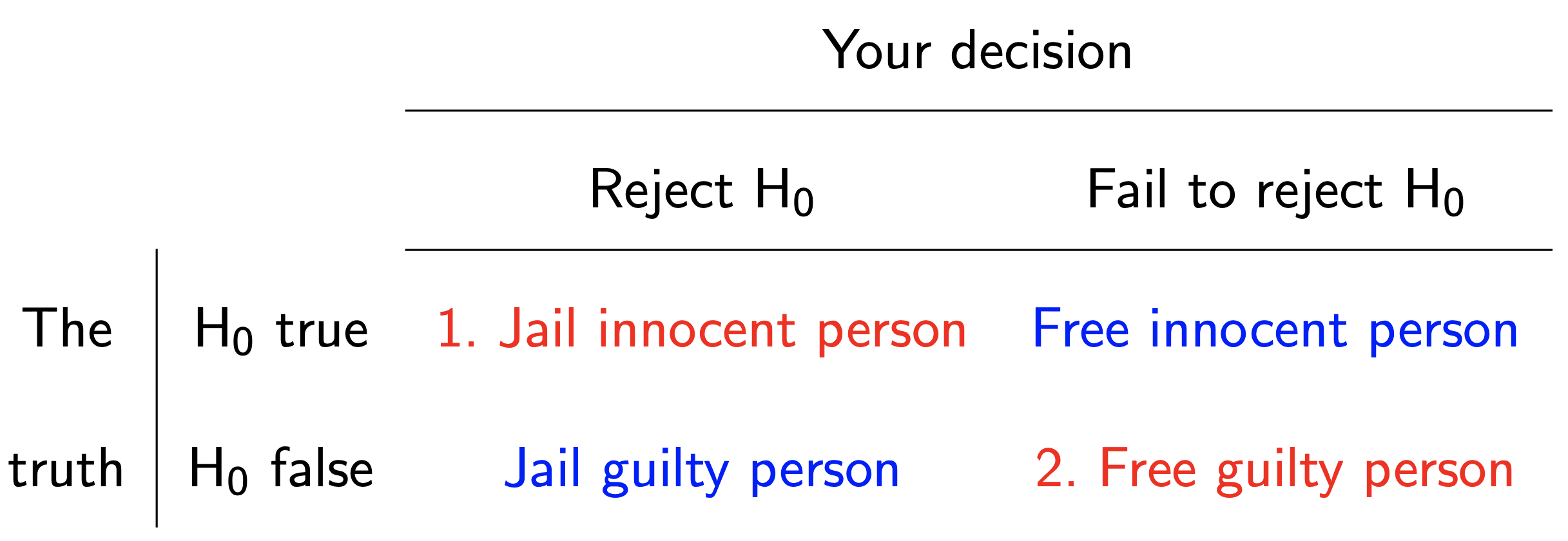
• Null hypothesis, \(H_0\): Defendant is innocent

• Alternative hypothesis, \(H_A\): Defendant is guilty

. . .

• Present the evidence: Collect data

. . .

• Judge the evidence: “Could these data plausibly have happened by chance if the null hypothesis were true?”
  • Yes: Fail to reject \(H_0\)
  • No: Reject \(H_0\)

Hypothesis testing as medical diagnosis

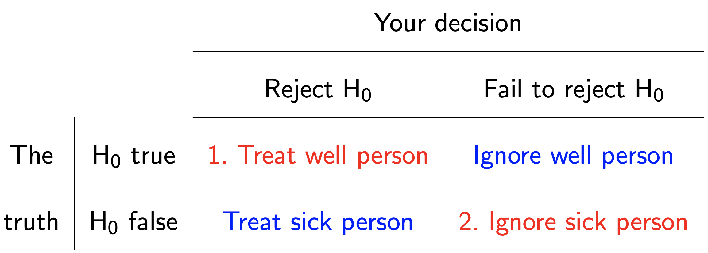
• Null hypothesis, \(H_0\): patient is fine

• Alternative hypothesis, \(H_A\): patient is sick

. . .

• Present the evidence: Collect data

. . .

• Judge the evidence: “Could these data plausibly have happened by chance if the null hypothesis were true?”
  • Yes: Fail to reject \(H_0\)
  • No: Reject \(H_0\)

Hypothesis testing framework

• Start with a null hypothesis, \(H_0\), that represents the status quo

• Set an alternative hypothesis, \(H_A\), that represents the research question, i.e. what we’re testing for

• Conduct a hypothesis test under the assumption that the null hypothesis is true and calculate a p-value (probability of observed or more extreme outcome given that the null hypothesis is true)

  • if the test results suggest that the data do not provide convincing evidence for the alternative hypothesis, stick with the null hypothesis
  • if they do, then reject the null hypothesis in favor of the alternative

Calculate observed slope

… which we have already done:

observed_fit <- duke_forest |>
  specify(price ~ area) |>
  fit()

observed_fit

# A tibble: 2 × 2
  term      estimate
  <chr>        <dbl>
1 intercept  116652.
2 area          159.

Simulate null distribution

set.seed(20250616)
null_dist <- duke_forest |>
  specify(price ~ area) |>
  hypothesize(null = "independence") |>
  generate(reps = 100, type = "permute") |>
  fit()

View null distribution

null_dist

# A tibble: 200 × 3
# Groups:   replicate [100]
   replicate term       estimate
       <int> <chr>         <dbl>
 1         1 intercept 500510.  
 2         1 area          21.4 
 3         2 intercept 569335.  
 4         2 area          -3.40
 5         3 intercept 528454.  
 6         3 area          11.3 
 7         4 intercept 518056.  
 8         4 area          15.1 
 9         5 intercept 637111.  
10         5 area         -27.8 
# ℹ 190 more rows

Visualize null distribution

null_dist |>
  filter(term == "area") |>
  ggplot(aes(x = estimate)) +
  geom_histogram(binwidth = 15)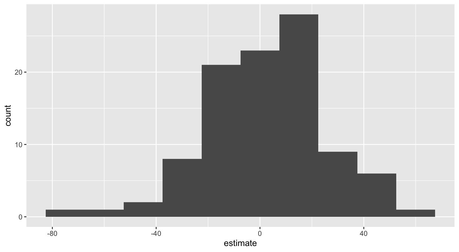

Visualize null distribution (alternative)

visualize(null_dist) +
  shade_p_value(obs_stat = observed_fit, direction = "two-sided")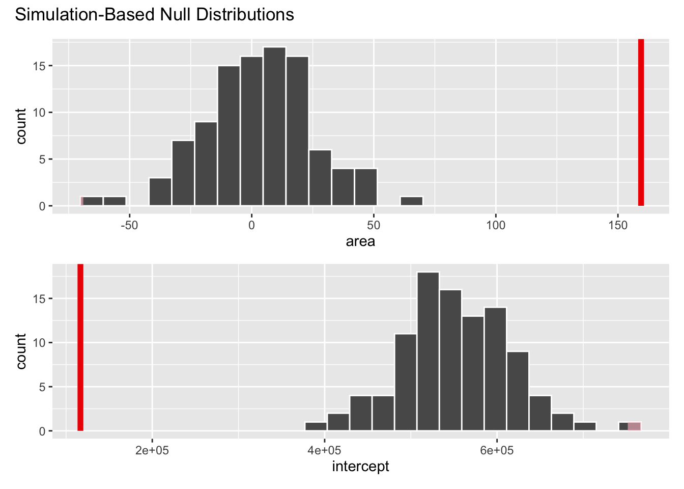

Get p-value

null_dist |>
  get_p_value(obs_stat = observed_fit, direction = "two-sided")

# A tibble: 2 × 2
  term      p_value
  <chr>       <dbl>
1 area            0
2 intercept       0

Make a decision

Based on the p-value calculated, what is the conclusion of the hypothesis test?

Sometimes the test will be wrong

• Type 1 error: False positive

• Type 2 error: False negative

Think about the judge

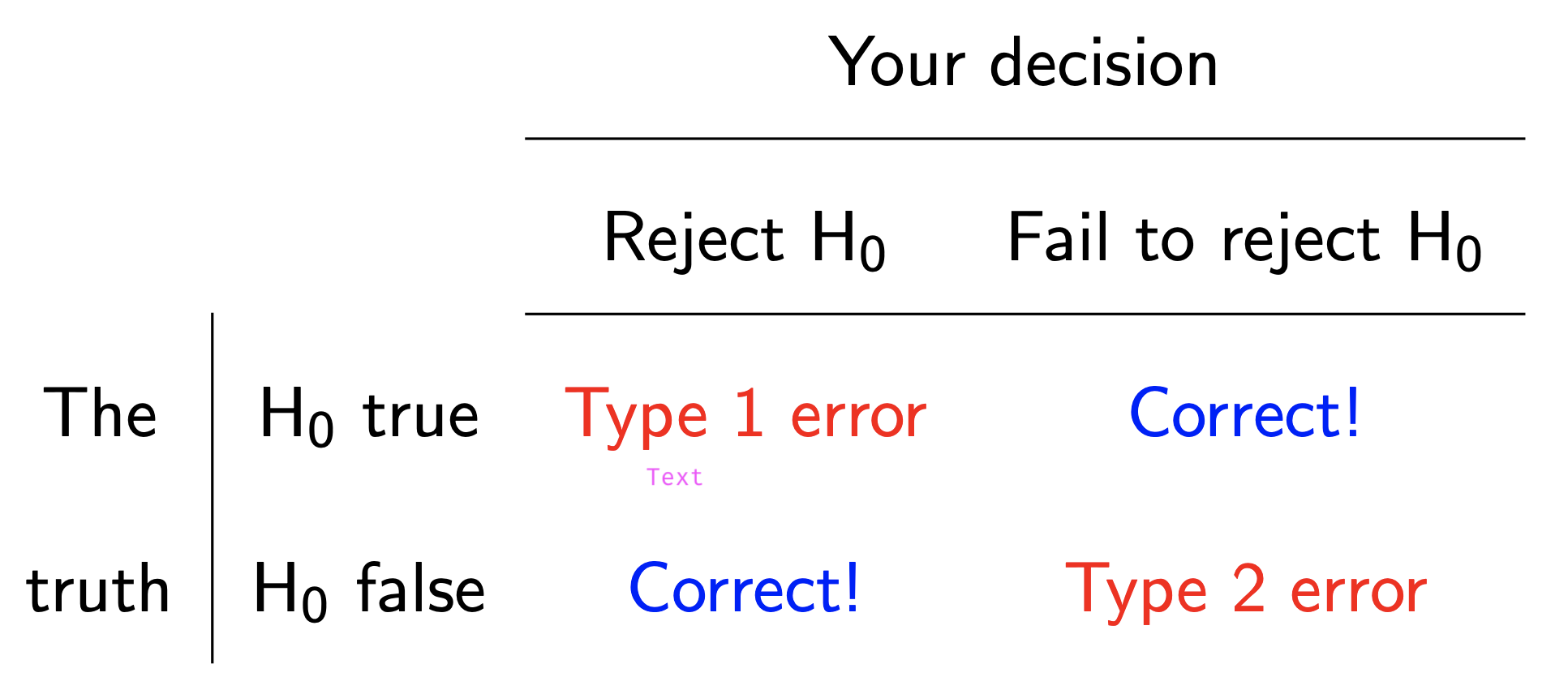
Which is worse, Type 1 or Type 2 error?

Note: \(H_0\) person innocent vs \(H_A\) person guilty.

. . .

Aspects of the American trial system regard a Type 1 error as worse than a Type 2 error (reasonable doubt standard, unanimous juries, presumption of innocence, etc).

Think about the doctor

Which is worse, Type 1 or Type 2 error? Which are doctors more prone to?

Note: \(H_0\) person well vs \(H_A\) person sick.

How do we negotiate the trade-off?

Pick a threshold \(\alpha\in[0,\,1]\) called the discernibility level and threshold the \(p\)-value:

• If \(p\text{-value} < \alpha\), reject null and find evidence for the alternative;
• If \(p\text{-value} \geq \alpha\), fail to reject null;

. . .

• \(\alpha\) \(\uparrow\) \(\rightarrow\) easier to reject \(H_0\) \(\rightarrow\) Type 1 \(\uparrow\) Type 2 \(\downarrow\)

• \(\alpha\) \(\downarrow\) \(\rightarrow\) harder to reject \(H_0\) \(\rightarrow\) Type 1 \(\downarrow\) Type 2 \(\uparrow\)

• Typical choices: \(\alpha\) = 0.01, 0.05, 0.10.