Hypothesis Testing

Lecture 21

June 16, 2025

While you wait…

Go to your ae project in RStudio.
Make sure all of your changes up to this point are committed and pushed, i.e., there’s nothing left in your Git pane.
Click Pull to get today’s application exercise file: ae-17-hypothesis-testing.qmd.
Wait till the you’re prompted to work on the application exercise during class before editing the file.

Recap: sampling uncertainty

What if this was my dataset?

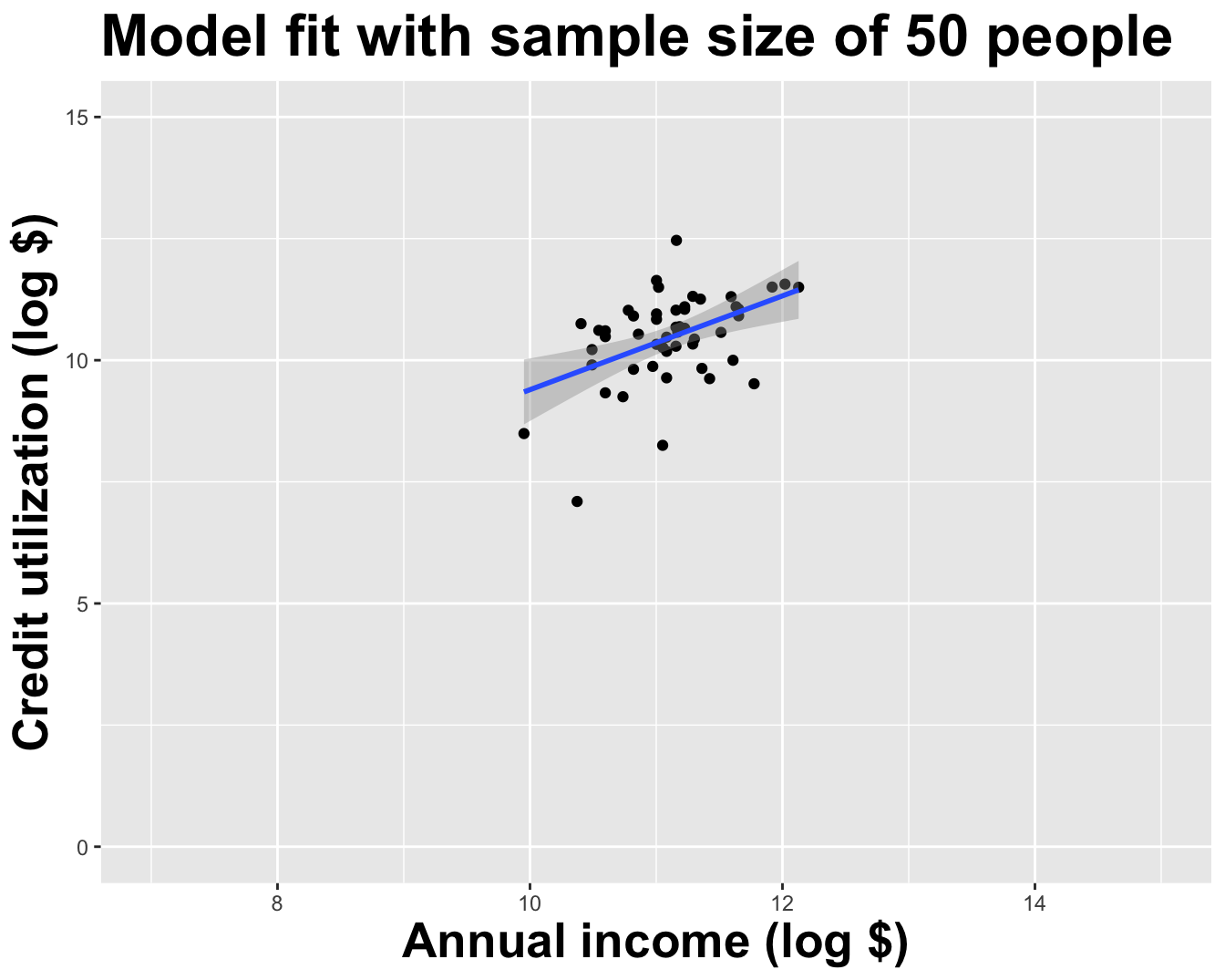
# A tibble: 2 × 2
  term        estimate
  <chr>          <dbl>
1 (Intercept)    2.56 
2 log_inc        0.718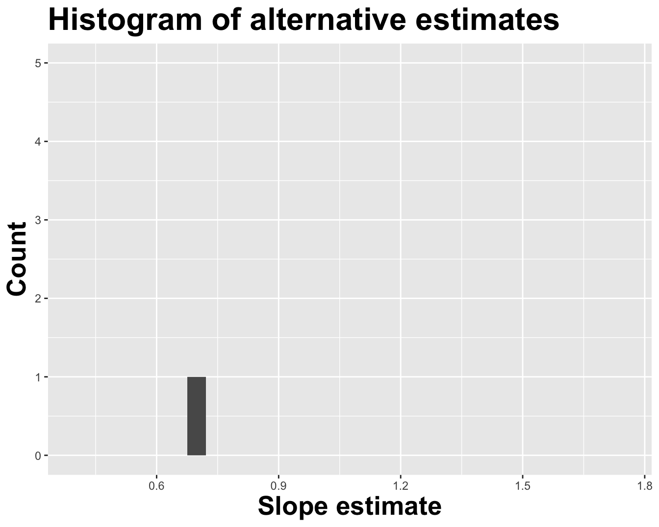

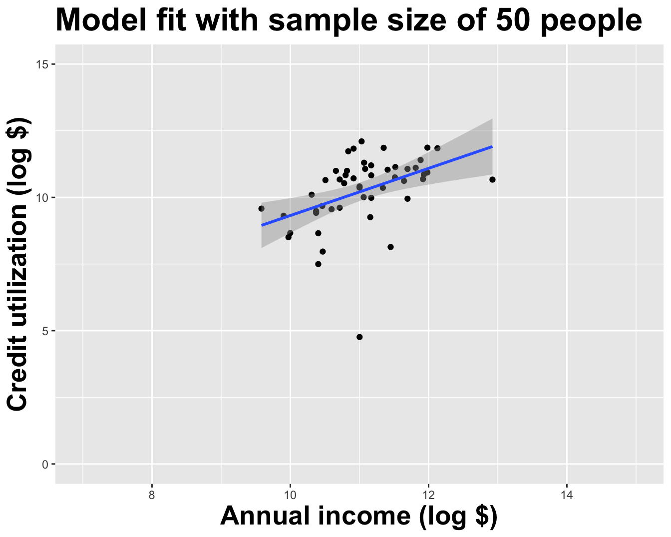
What if this was my dataset instead?

# A tibble: 2 × 2
  term        estimate
  <chr>          <dbl>
1 (Intercept)   -0.250
2 log_inc        0.964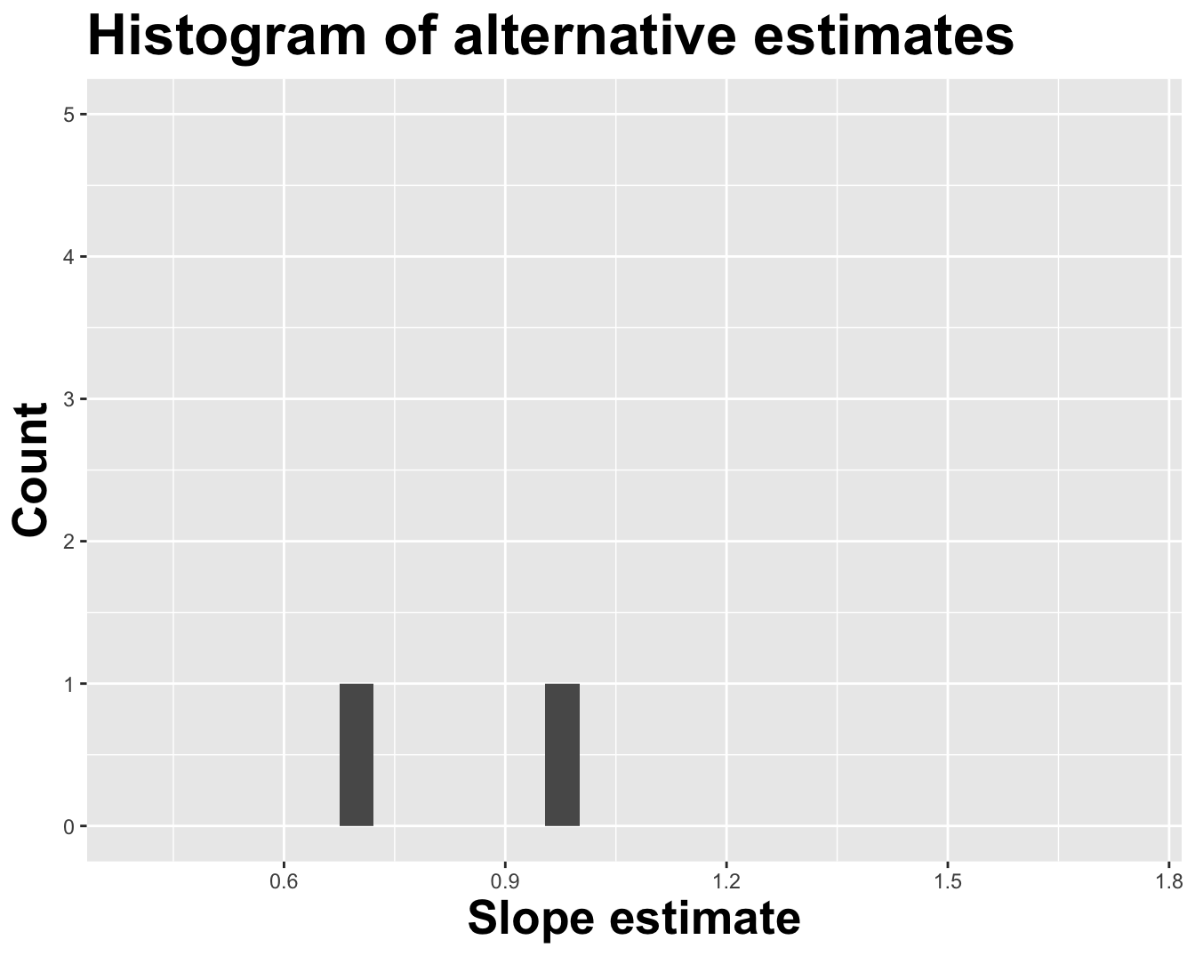

What if this was my dataset instead?

# A tibble: 2 × 2
  term        estimate
  <chr>          <dbl>
1 (Intercept)    0.468
2 log_inc        0.885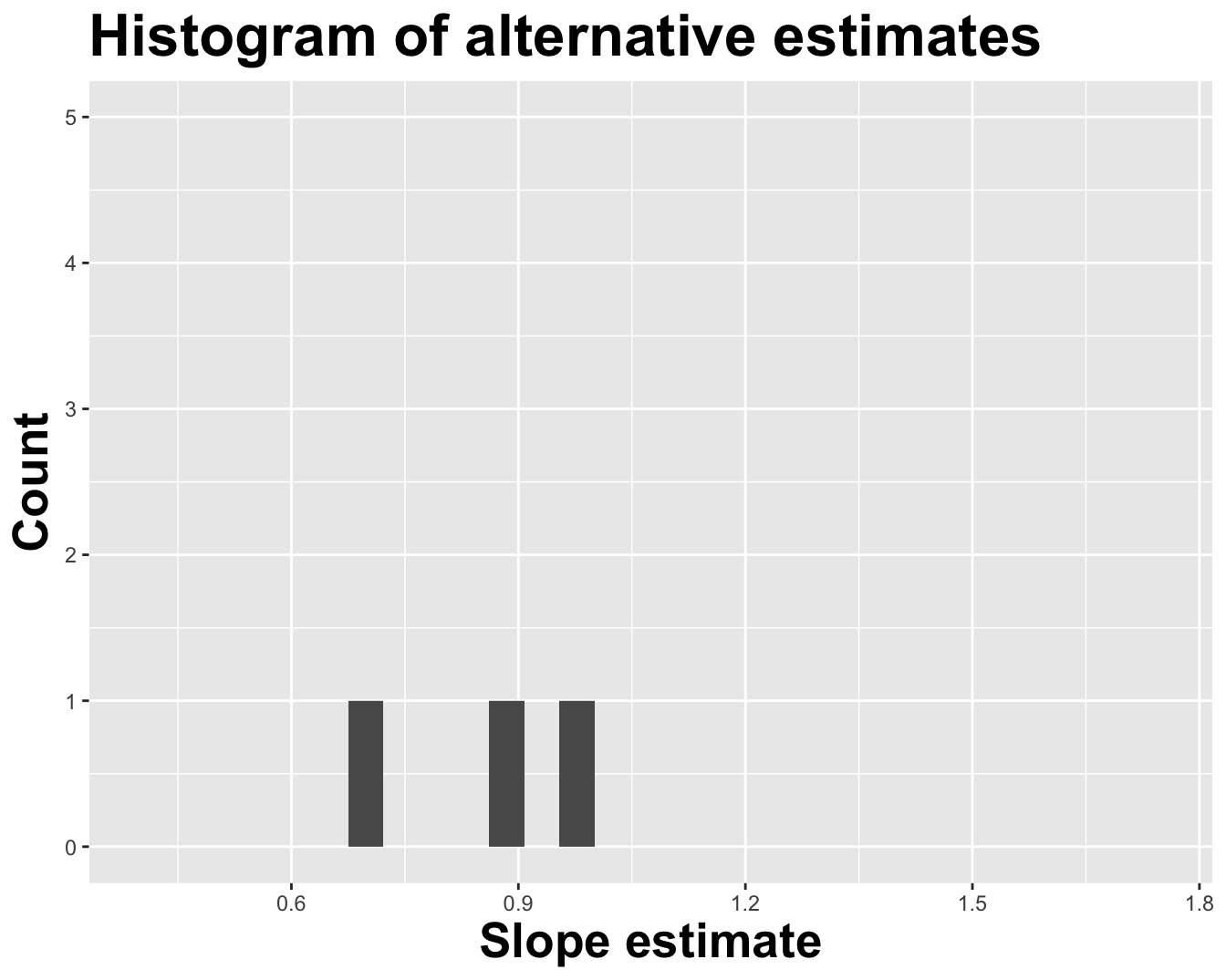

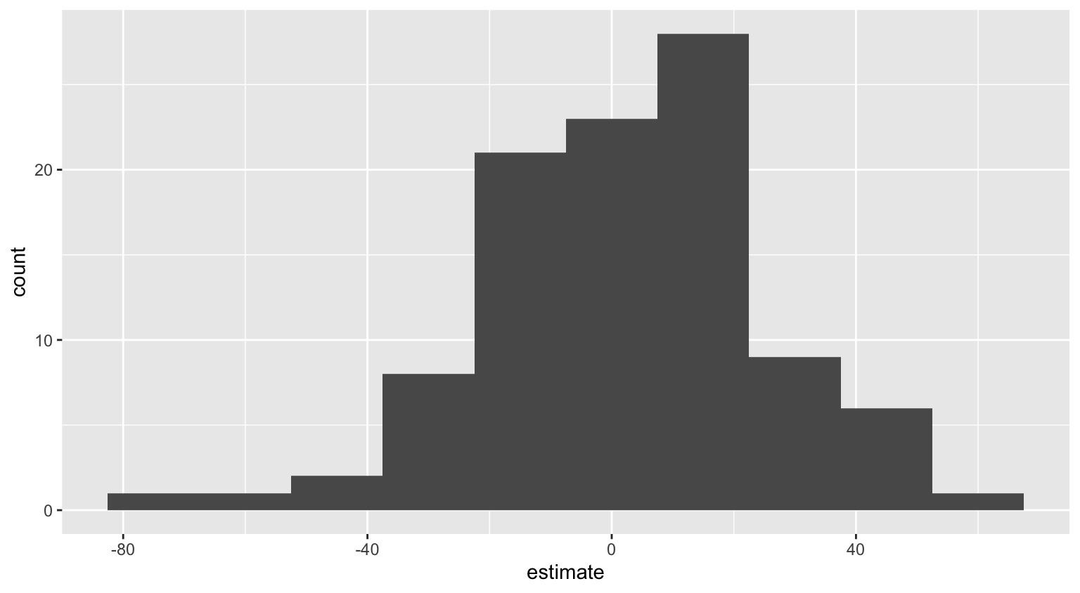
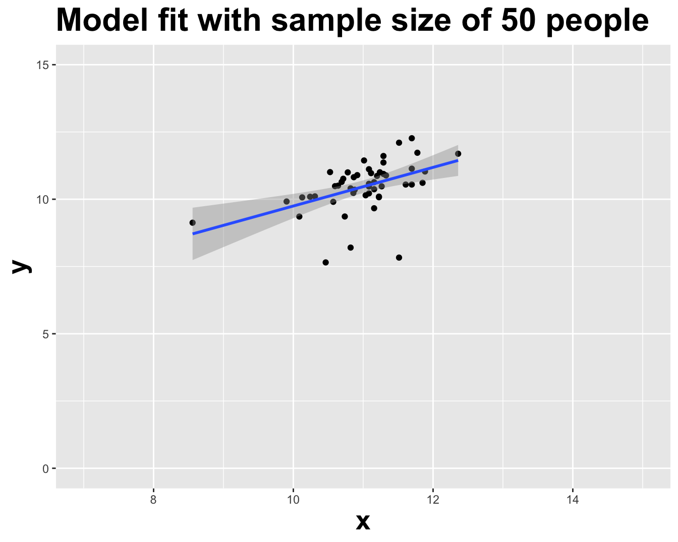
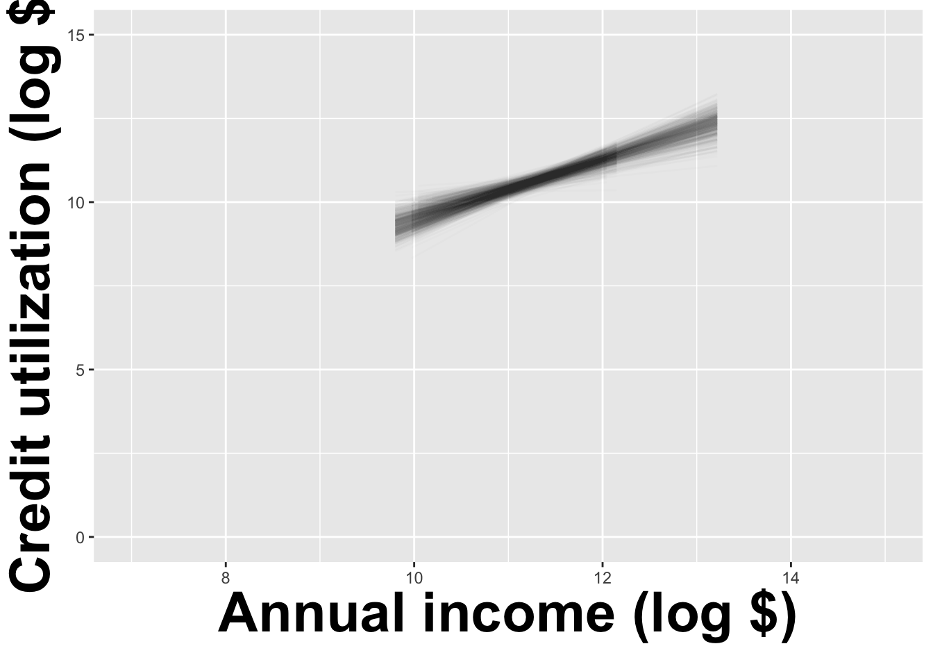
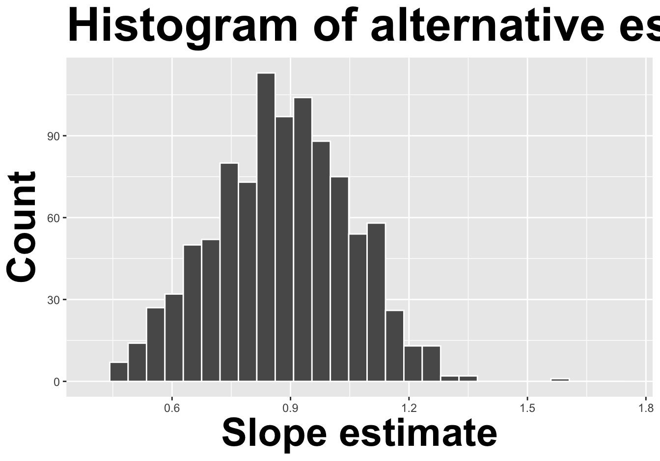
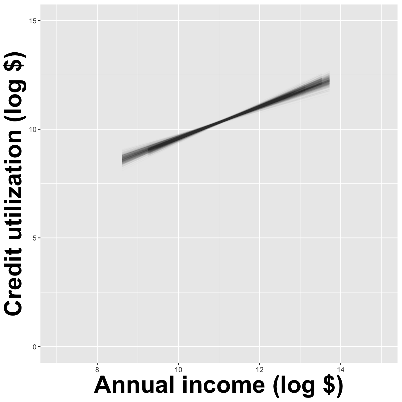
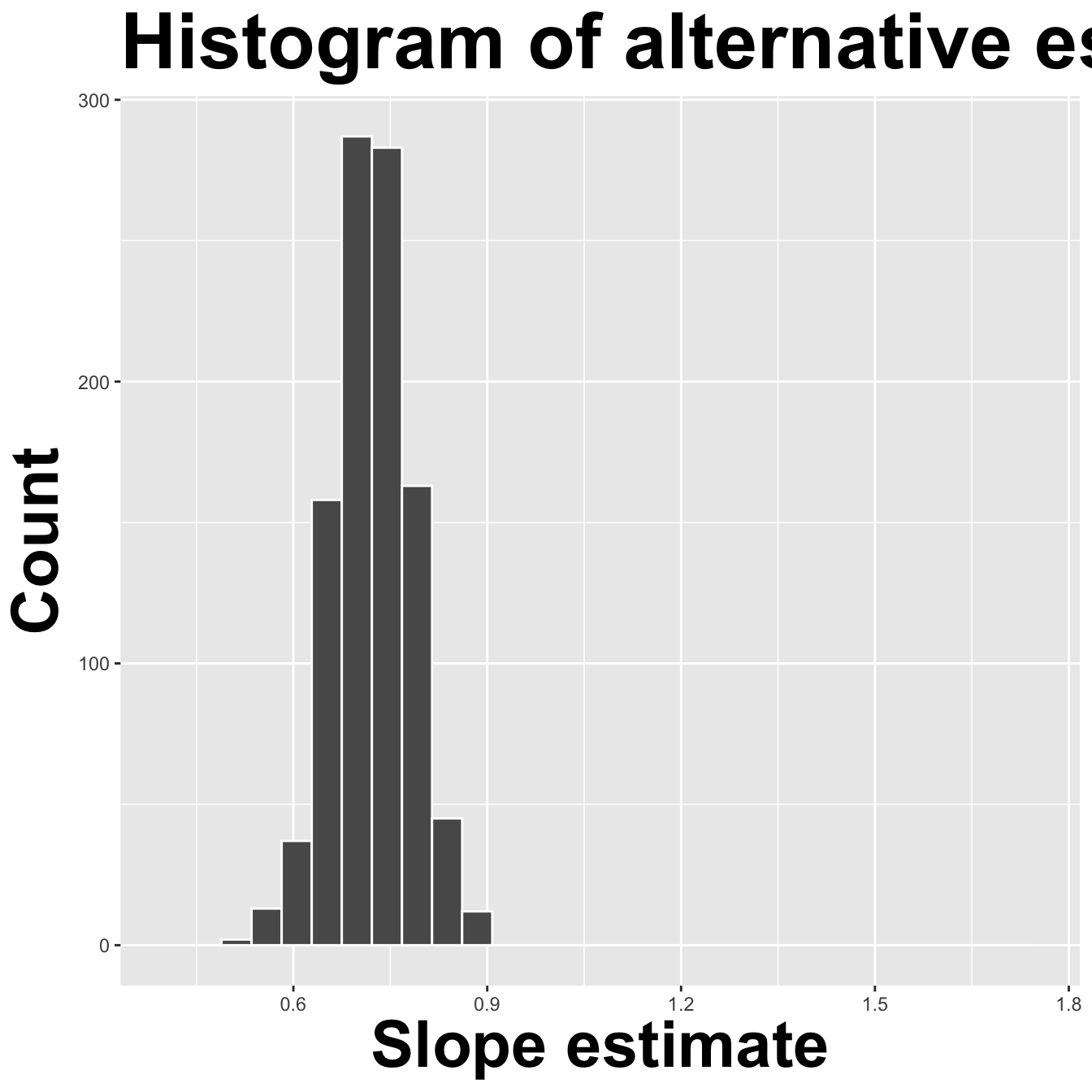
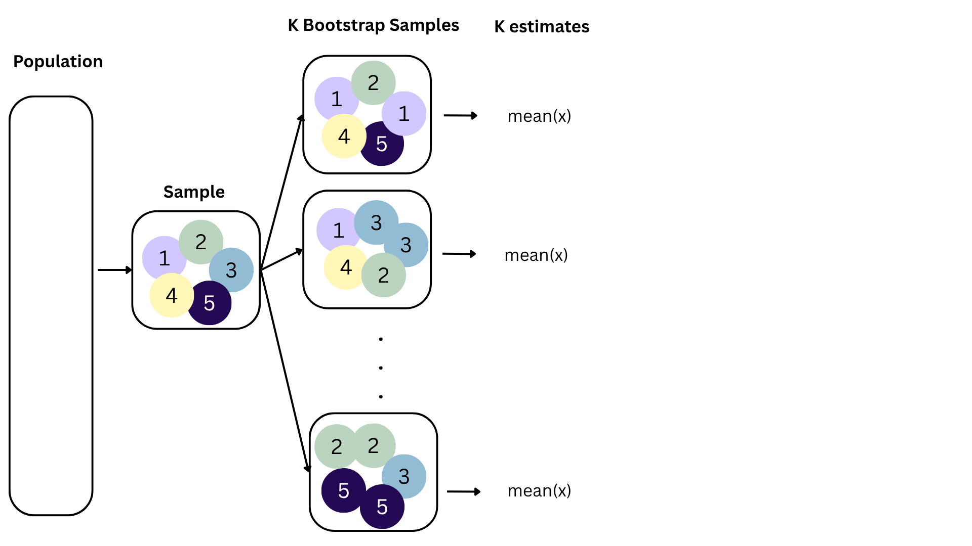
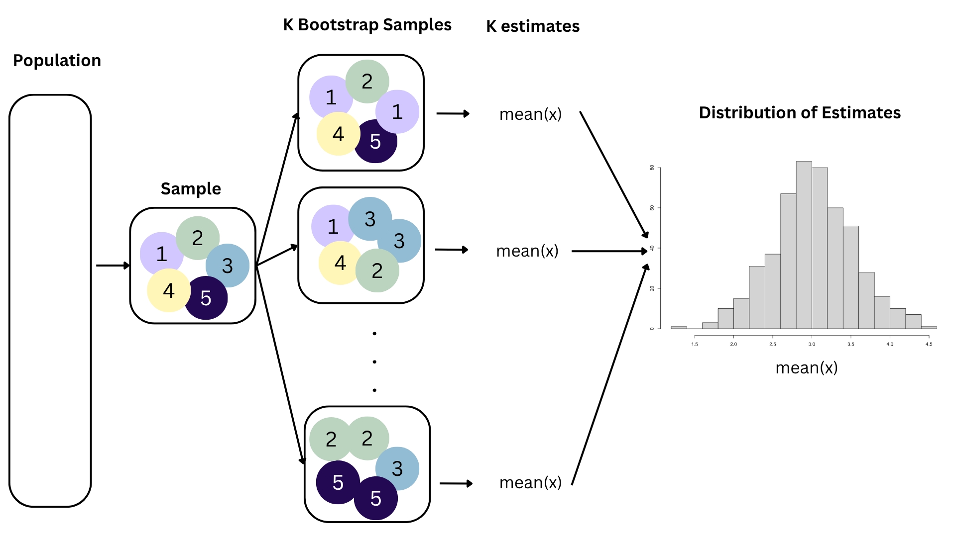
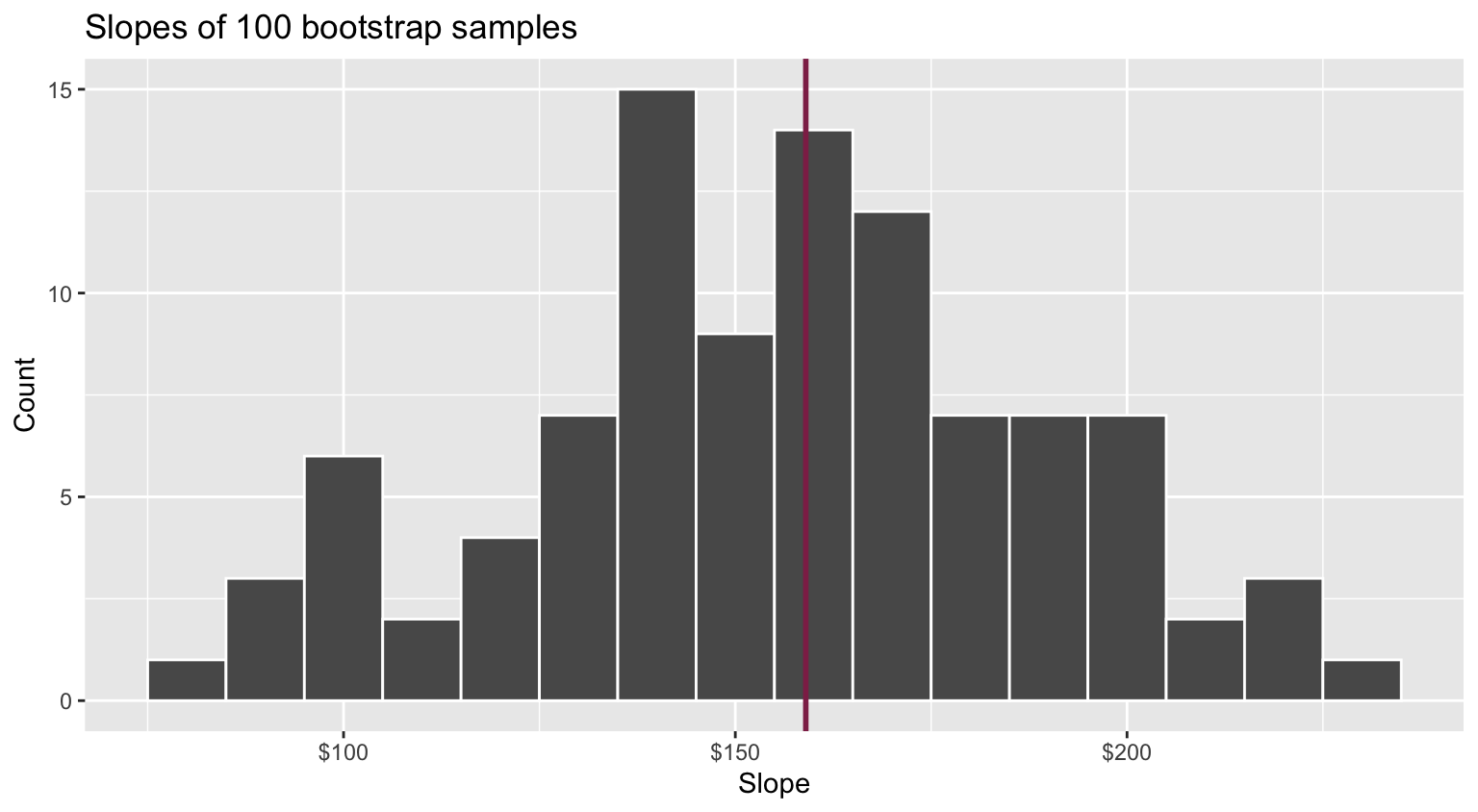
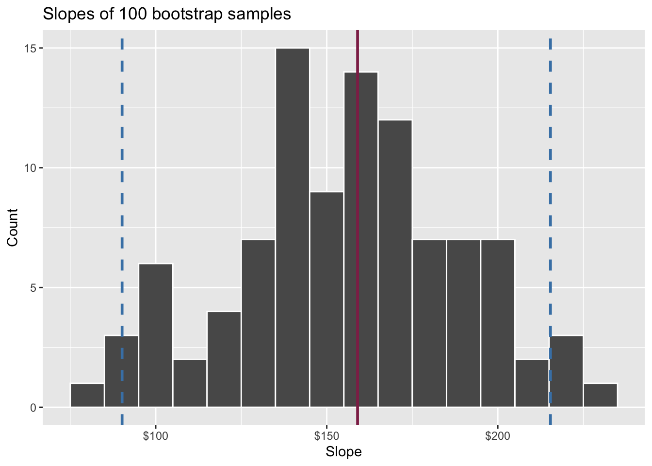
Rinse and repeat 1000 times…

Sampling uncertainty

How sensitive are the estimates to the data they are based on?

Very? Then uncertainty is high, results are unreliable;
Not very? Uncertainty is low, results are more reliable.

That was for n = 50. What if I was starting with n = 1000?

Sampling uncertainty decreased!

Bootstrapping

Data collection is costly, so we have to do our best with what we already have;
We approximate this idea of “alternative, hypothetical datasets I could have observed” by resampling our data with replacement;
We construct a new dataset of the same size by randomly picking rows out of the original one:
- Some rows will be duplicated;
- Some rows will not appear at all;
- The new dataset is different from the original;
- Different dataset >> different estimate
Repeat this processes hundred or thousands of times, and observe how the estimates vary as you refit the model on alternative datasets.
This gives you a sense of the sampling variability of your estimates.

Bootstrapping Procedure

Bootstrapping

Bootstrapping

Bootstrapping

Bootstrapping

Bootstrapping

Bootstrapping

Confidence intervals

Point estimation: report your single number best guess for the unknown quantity;
Interval estimation: report a range, or interval, or values where you think the unknown quantity is likely to live;
- Interval should be wide enough to capture the truth with high probability;
- Interval should be narrow enough to be informative;
Unfortunately, there is a trade-off. You adjust the confidence level to try to negotiate the trade-off;
Common choices: 90%, 95%, 99%.

Precision vs. accuracy

Recap: Computing Confidence Interval

Friday’s Data: Houses in Duke Forest

Data on houses that were sold in the Duke Forest neighborhood of Durham, NC around November 2020
Scraped from Zillow
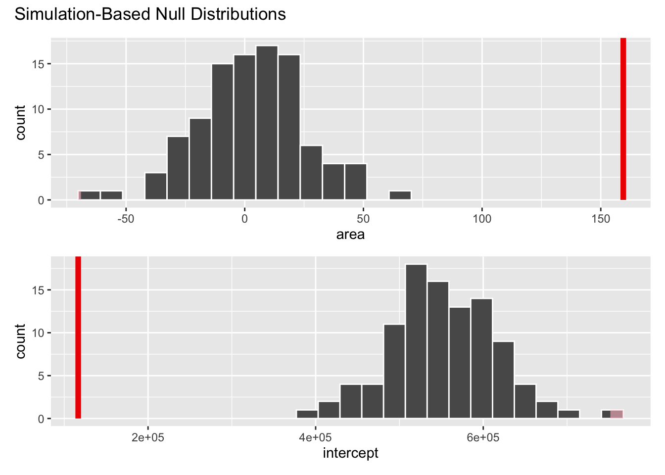
Source: openintro::duke_forest

Home in Duke Forest

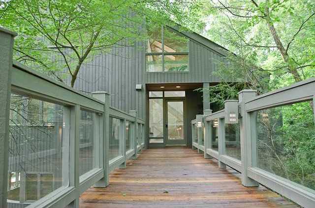
Goal: Use the area (in square feet) to understand variability in the price of houses in Duke Forest.

Point Estimate

observed_fit <- duke_forest |>
  specify(price ~ area) |>
  fit()

observed_fit

# A tibble: 2 × 2
  term      estimate
  <chr>        <dbl>
1 intercept  116652.
2 area          159.

Slopes of bootstrap samples

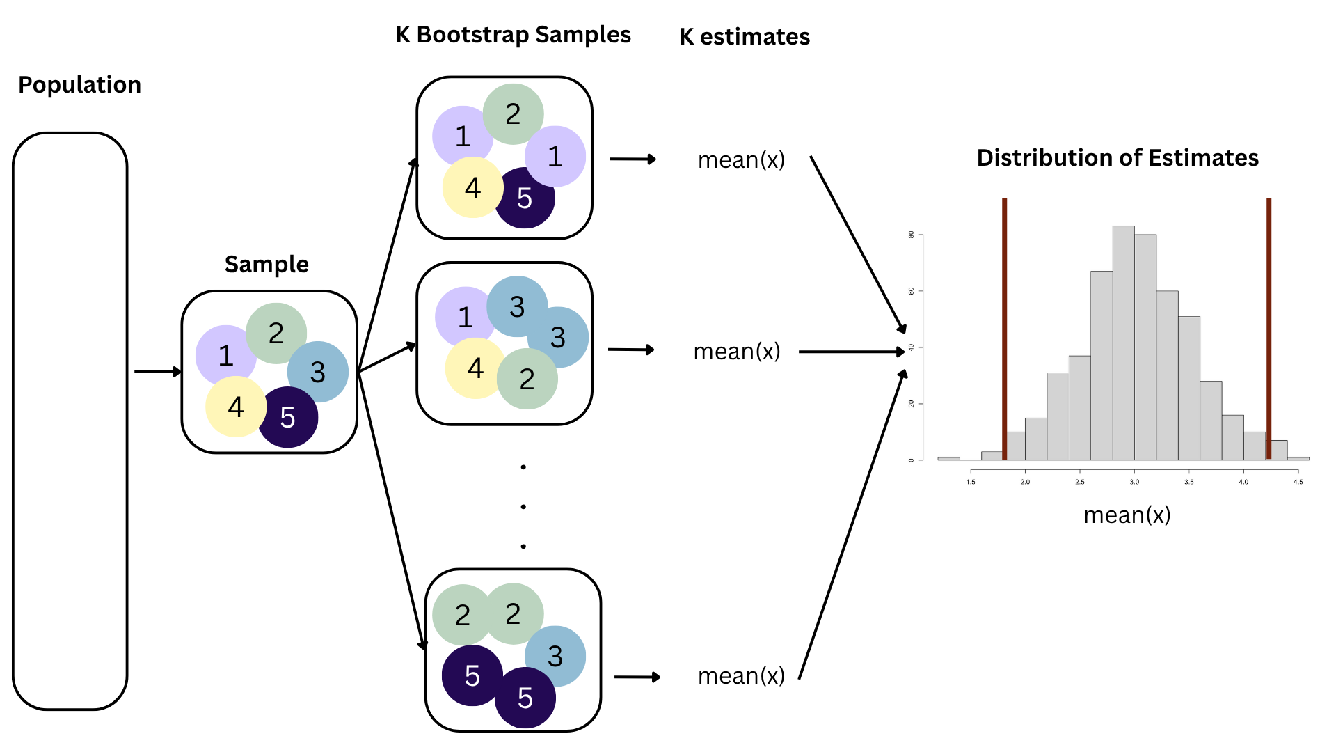
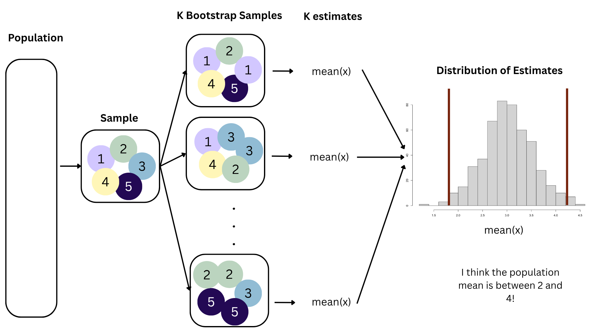
Fill in the blank: For each additional square foot, the model predicts the sale price of Duke Forest houses to be higher, on average, by between ___ and ___ dollars.

Slopes of bootstrap samples

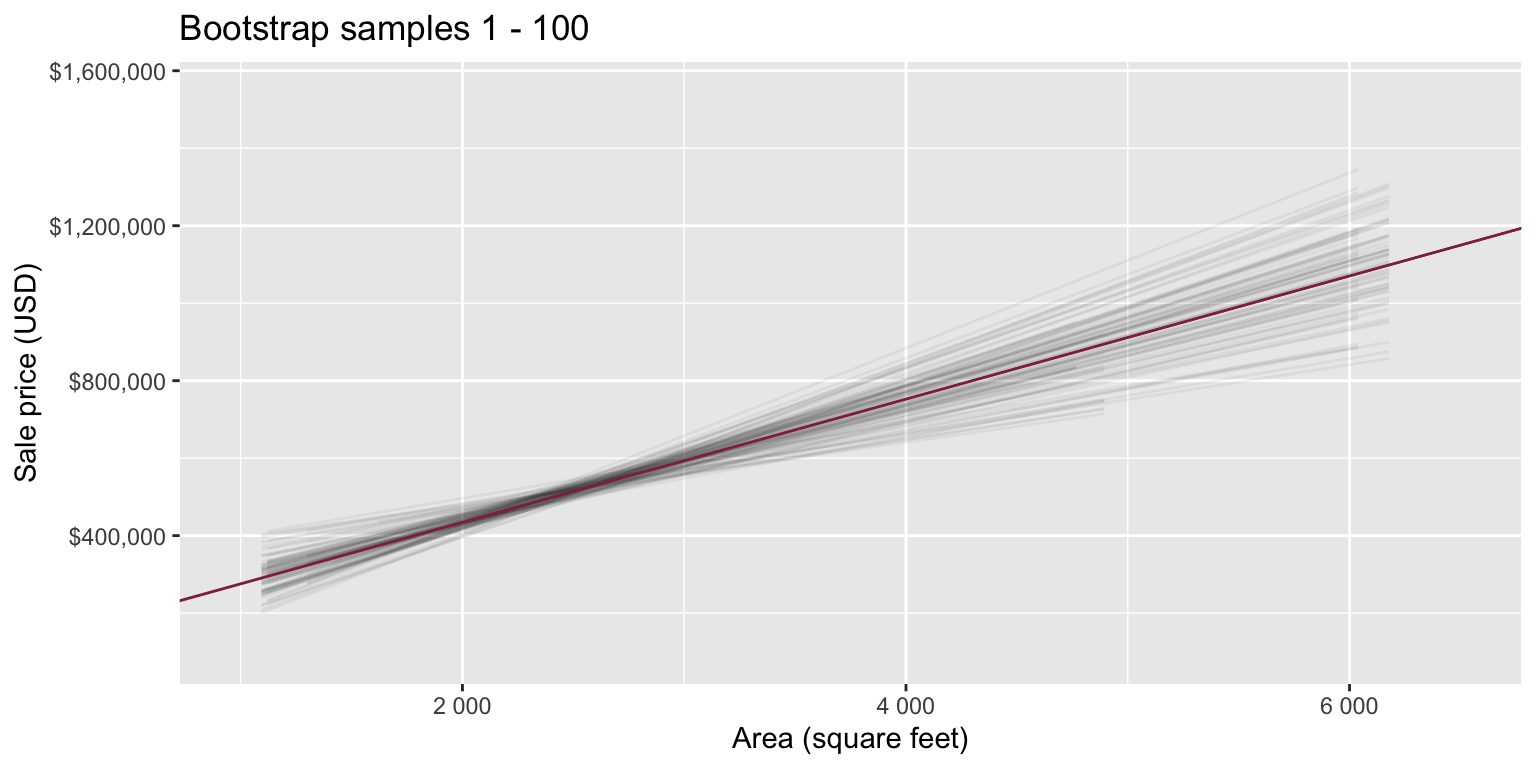
Fill in the blank: For each additional square foot, we expect the sale price of Duke Forest houses to be higher, on average, by between ___ and ___ dollars.

95% confidence interval

A 95% confidence interval is bounded by the middle 95% of the bootstrap distribution
We are 95% confident that for each additional square foot, the model predicts the sale price of Duke Forest houses to be higher, on average, by $90.17 to $215.39.

Where do the bounds come from?

Think IQR! 50% of the bootstrap distribution is between the 25% quantile on the left and the 75% quantile on the right. But we want more than 50%
90% of the bootstrap distribution is between the 5% quantile on the left and the 95% quantile on the right;
95% of the bootstrap distribution is between the 2.5% quantile on the left and the 97.5% quantile on the right;
And so on.

Recap (again!!)

Population: Complete set of observations of whatever we are studying, e.g., people, tweets, photographs, etc. (population size = $N$)
Sample: Subset of the population, ideally random and representative (sample size = $n$)
Sample statistic $\ne$ population parameter, but if the sample is good, it can be a good estimate
Statistical inference: Discipline that concerns itself with the development of procedures, methods, and theorems that allow us to extract meaning and information from data that has been generated by stochastic (random) process
We report the estimate with a confidence interval, and the width of this interval depends on the variability of sample statistics from different samples from the population
Since we can’t continue sampling from the population, we bootstrap from the one sample we have to estimate sampling variability

Hypothesis testing

A hypothesis test is a statistical technique used to evaluate competing claims using data

Null hypothesis, $H_0$: An assumption about the population. “There is nothing going on.”
Alternative hypothesis, $H_A$: A research question about the population. “There is something going on”.

Note: Hypotheses are always at the population level!

Setting hypotheses

Null hypothesis, $H_0$: “There is nothing going on.” The slope of the model for predicting the prices of houses in Duke Forest from their areas is 0, $\beta_1 = 0$.
Alternative hypothesis, $H_A$: “There is something going on”. The slope of the model for predicting the prices of houses in Duke Forest from their areas is different than, $\beta_1 \ne 0$.

Hypothesis testing “mindset”

Assume you live in a world where null hypothesis is true: $\beta_1 = 0$.
Ask yourself how likely you are to observe the sample statistic, or something even more extreme, in this world: $P(b_1 \leq 159.48~or~b_1 \geq 159.48 | \beta_1 = 0)$ = ?

Hypothesis testing as a court trial

Null hypothesis, $H_0$: Defendant is innocent
Alternative hypothesis, $H_A$: Defendant is guilty

Present the evidence: Collect data

Judge the evidence: “Could these data plausibly have happened by chance if the null hypothesis were true?”
- Yes: Fail to reject $H_0$
- No: Reject $H_0$

Hypothesis testing as medical diagnosis

Null hypothesis, $H_0$: patient is fine
Alternative hypothesis, $H_A$: patient is sick

Present the evidence: Collect data

Judge the evidence: “Could these data plausibly have happened by chance if the null hypothesis were true?”
- Yes: Fail to reject $H_0$
- No: Reject $H_0$

Hypothesis testing framework

Start with a null hypothesis, $H_0$, that represents the status quo
Set an alternative hypothesis, $H_A$, that represents the research question, i.e. what we’re testing for
Conduct a hypothesis test under the assumption that the null hypothesis is true and calculate a p-value (probability of observed or more extreme outcome given that the null hypothesis is true)
- if the test results suggest that the data do not provide convincing evidence for the alternative hypothesis, stick with the null hypothesis
- if they do, then reject the null hypothesis in favor of the alternative

Calculate observed slope

… which we have already done:

observed_fit <- duke_forest |>
  specify(price ~ area) |>
  fit()

observed_fit

# A tibble: 2 × 2
  term      estimate
  <chr>        <dbl>
1 intercept  116652.
2 area          159.

Simulate null distribution

set.seed(20250616)
null_dist <- duke_forest |>
  specify(price ~ area) |>
  hypothesize(null = "independence") |>
  generate(reps = 100, type = "permute") |>
  fit()

View null distribution

null_dist

# A tibble: 200 × 3
# Groups:   replicate [100]
   replicate term       estimate
       <int> <chr>         <dbl>
 1         1 intercept 500510.  
 2         1 area          21.4 
 3         2 intercept 569335.  
 4         2 area          -3.40
 5         3 intercept 528454.  
 6         3 area          11.3 
 7         4 intercept 518056.  
 8         4 area          15.1 
 9         5 intercept 637111.  
10         5 area         -27.8 
# ℹ 190 more rows

Visualize null distribution

null_dist |>
  filter(term == "area") |>
  ggplot(aes(x = estimate)) +
  geom_histogram(binwidth = 15)

Visualize null distribution (alternative)

visualize(null_dist) +
  shade_p_value(obs_stat = observed_fit, direction = "two-sided")

Get p-value

null_dist |>
  get_p_value(obs_stat = observed_fit, direction = "two-sided")

# A tibble: 2 × 2
  term      p_value
  <chr>       <dbl>
1 area            0
2 intercept       0

Make a decision

Based on the p-value calculated, what is the conclusion of the hypothesis test?

Sometimes the test will be wrong

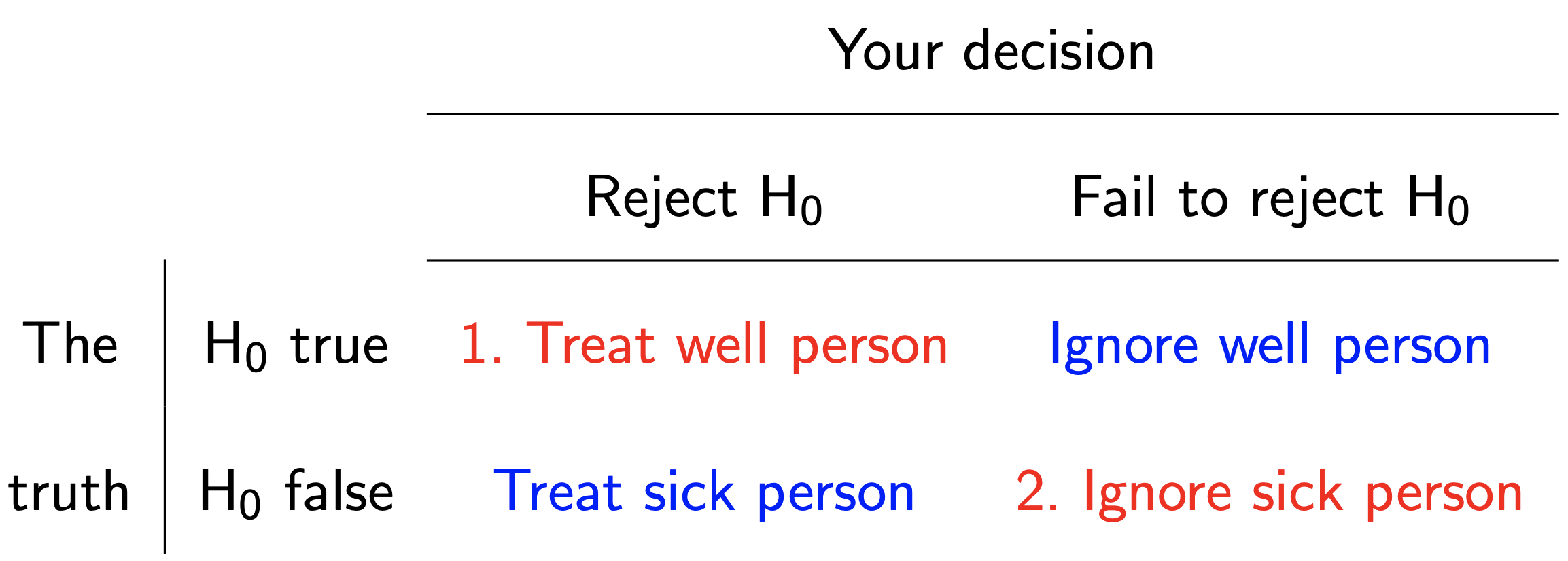
Type 1 error: False positive
Type 2 error: False negative

Think about the judge

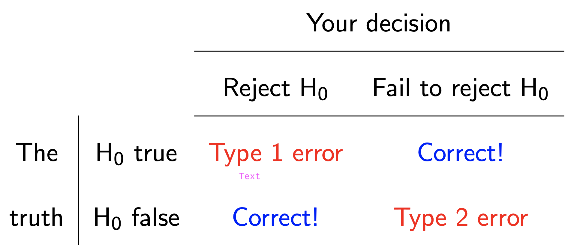
Which is worse, Type 1 or Type 2 error?

Note: $H_0$ person innocent vs $H_A$ person guilty.

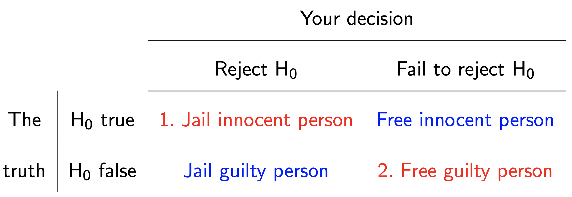
Aspects of the American trial system regard a Type 1 error as worse than a Type 2 error (reasonable doubt standard, unanimous juries, presumption of innocence, etc).

Think about the doctor

Which is worse, Type 1 or Type 2 error? Which are doctors more prone to?

Note: $H_0$ person well vs $H_A$ person sick.

How do we negotiate the trade-off?

Pick a threshold $\alpha\in[0,\,1]$ called the discernibility level and threshold the $p$-value:

If $p\text{-value} < \alpha$, reject null and find evidence for the alternative;
If $p\text{-value} \geq \alpha$, fail to reject null;

$\alpha$ $\uparrow$ $\rightarrow$ easier to reject $H_0$ $\rightarrow$ Type 1 $\uparrow$ Type 2 $\downarrow$
$\alpha$ $\downarrow$ $\rightarrow$ harder to reject $H_0$ $\rightarrow$ Type 1 $\downarrow$ Type 2 $\uparrow$
Typical choices: $\alpha$ = 0.01, 0.05, 0.10.