Quantifying uncertainty with bootstrap intervals
Lecture 20
Announcements
Project timeline and progress:
-
Due TONIGHT: Milestone 3
- Address and close issues (let me know if you are having trouble closing!)
- At least one plot
- All team members commit
-
Before Monday - Between Milestones 3 and 4
- Make real progress on your project write-up: introduction and exploratory data analysis; brainstorm of methods you plan to use
- Ideal: Start trying the methods!
-
On Monday - Milestone 4
- First 30 mins: talk/work as teams
- Last 45 mins: give feedback to another team!
Yesterday was a lot…
Quick Recap!
Confusion Matrix
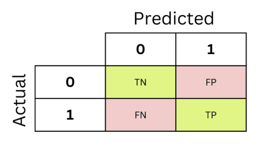
- False negative rate = \(\frac{FN}{FN + TP}\)
- False positive rate = \(\frac{FP}{FP + TN}\)
- Sensitivity = \(\frac{FN}{FN + TP}\) = 1 − False negative rate
- Specificity = \(\frac{TN}{FP + TN}\) = 1 - False positive rate
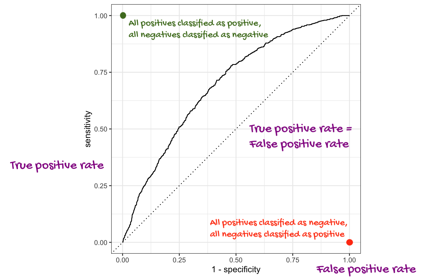
ROC Curve
Quantifying uncertainty
Samples
Generally, we don’t have information about an entire population, we have data for a sample:
Election polling: we can’t ask everybody who they are voting for
Housing data: we don’t have a data set with every single house
Medical research: we don’t test a new drug on everyone, just on a sample of patients in a clinical trial.
Ecology studies: scientists might analyze a smaller sample of animals/plants
. . .
There is uncertainty about true population parameters.
Statistical inference
Statistical inference provide methods and tools so we can use the single observed sample to make valid statements (inferences) about the population it comes from
For our inferences to be valid, the sample should be random and representative of the population we’re interested in
Example - Means
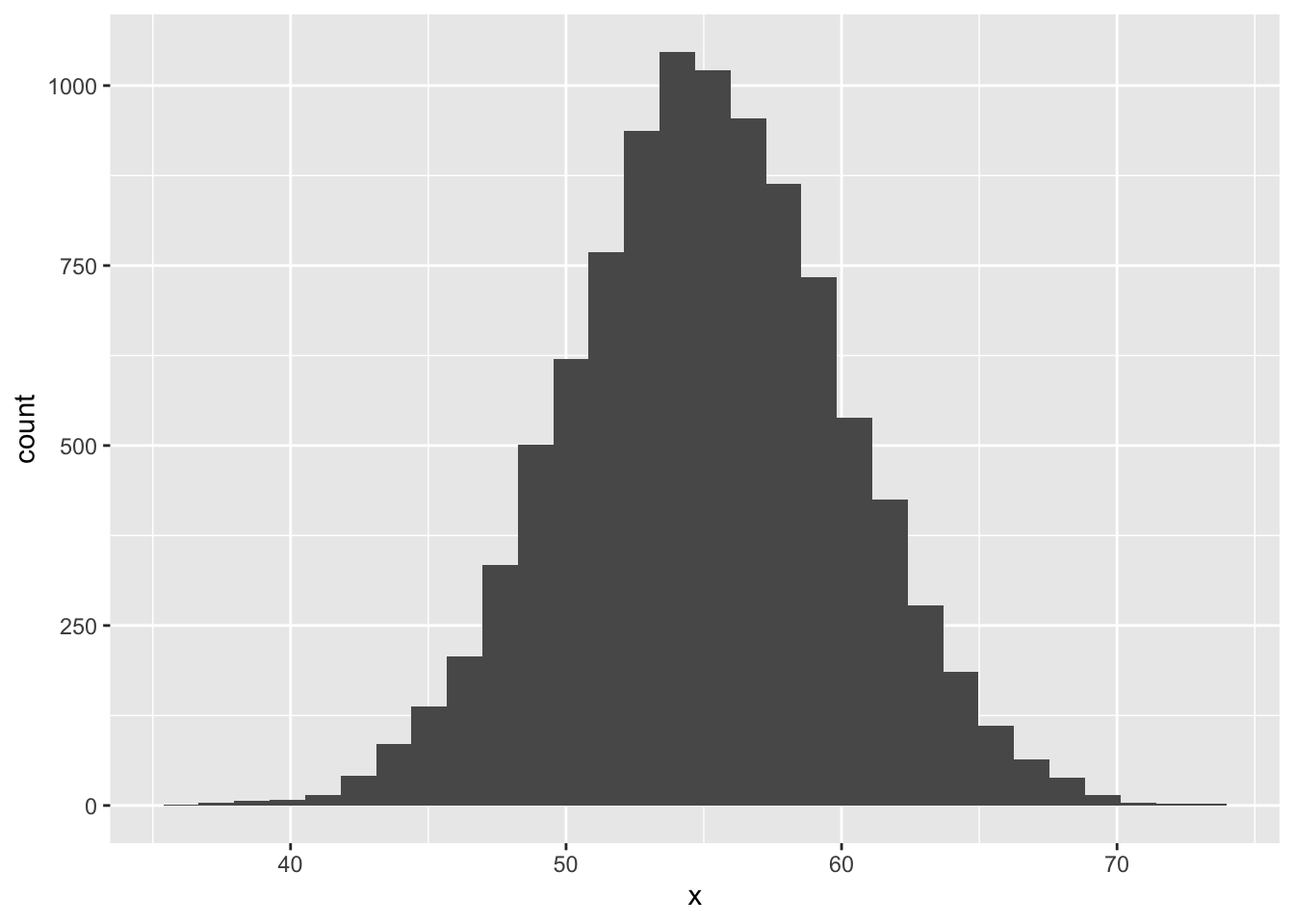
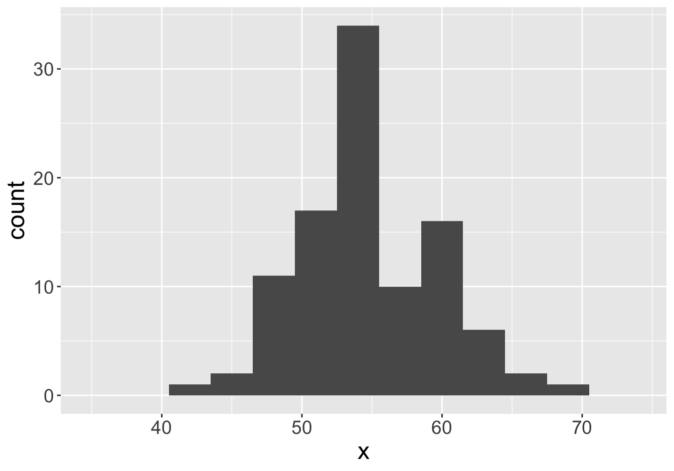
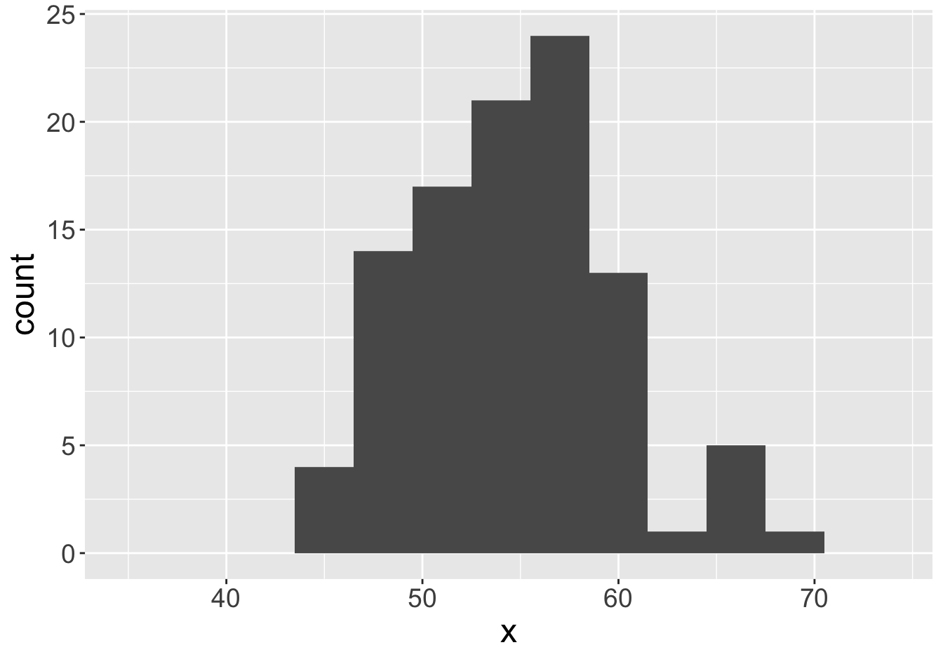
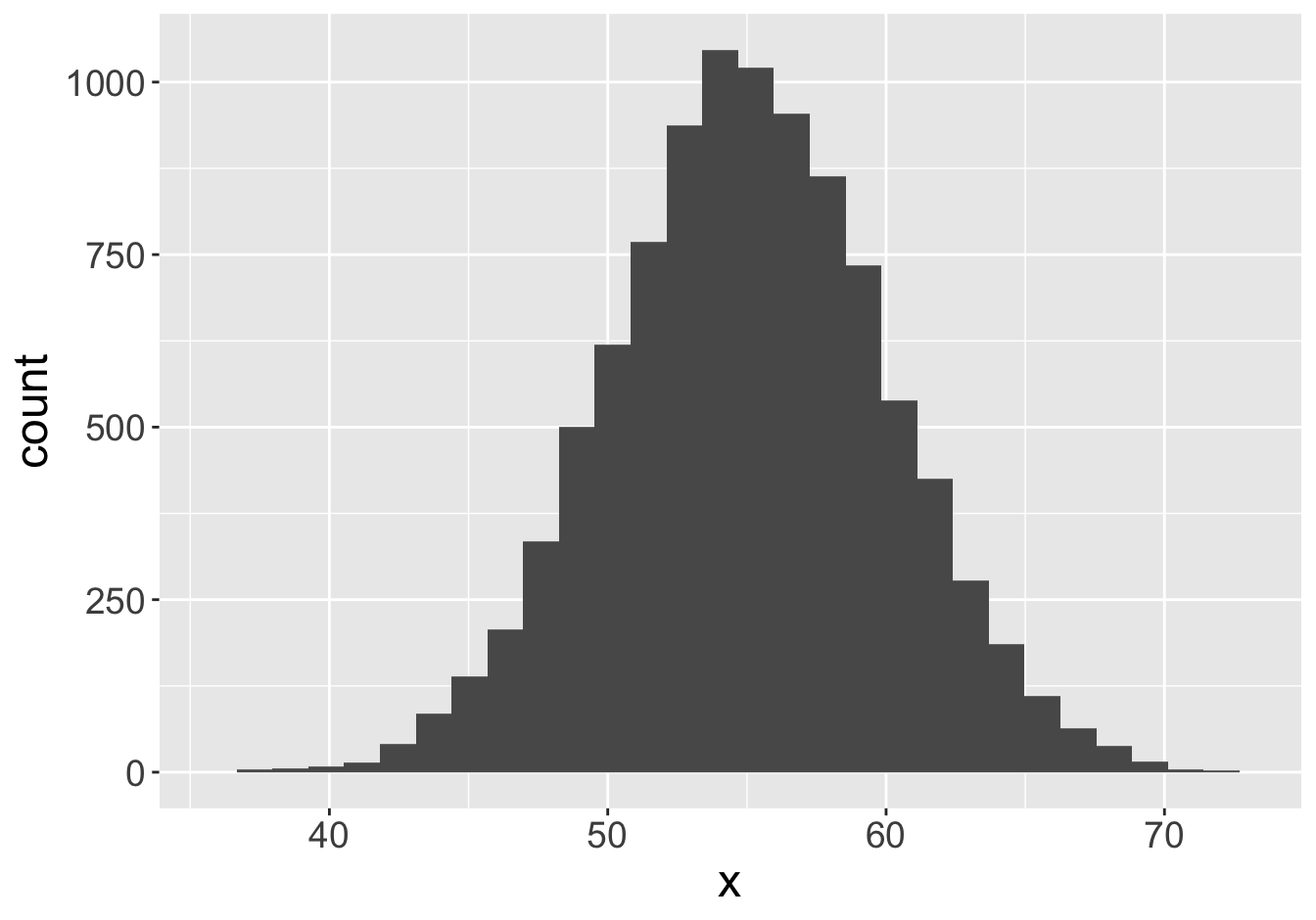
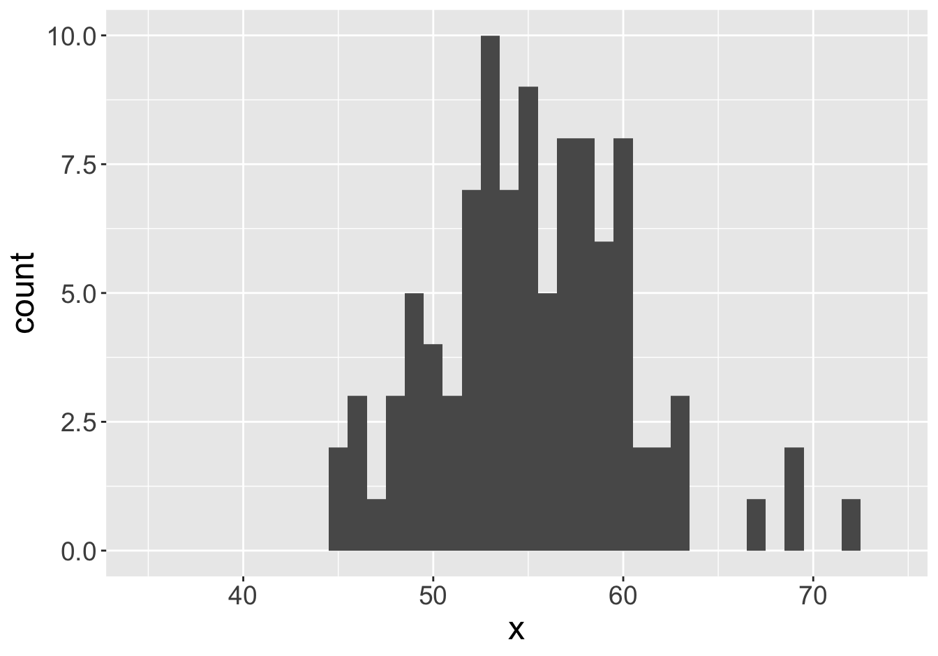
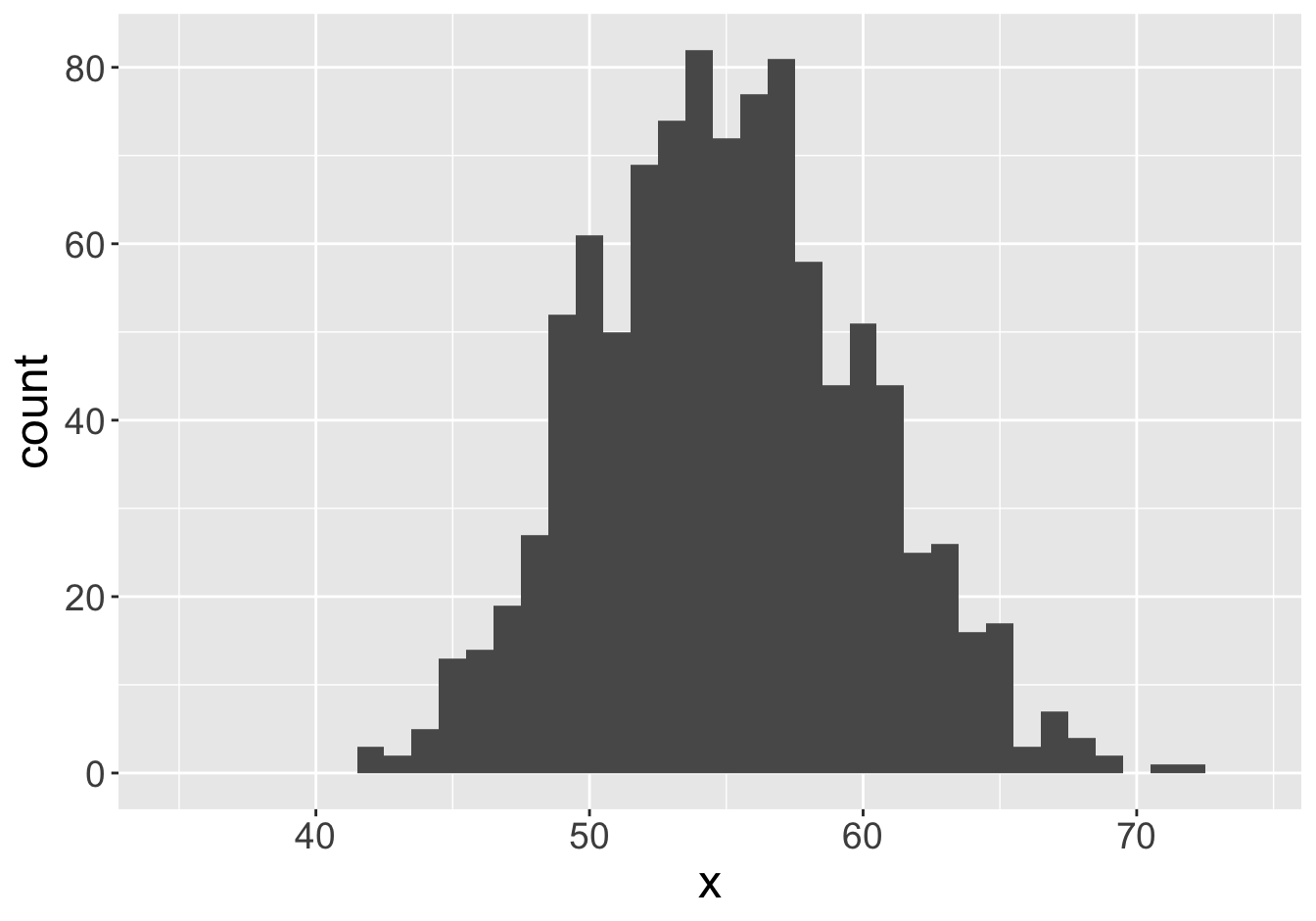
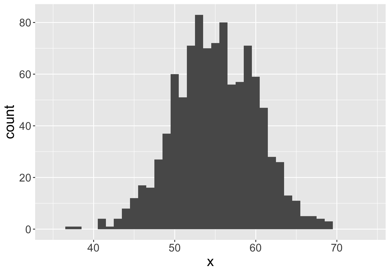
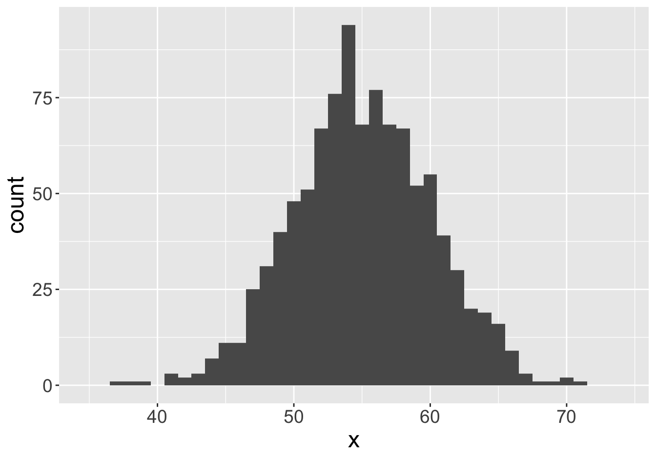
Suppose this histogram represents some value \(x\) in a population of 10,000:
Mean: 55.06
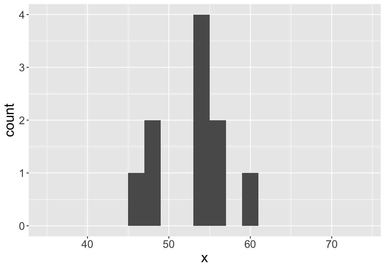
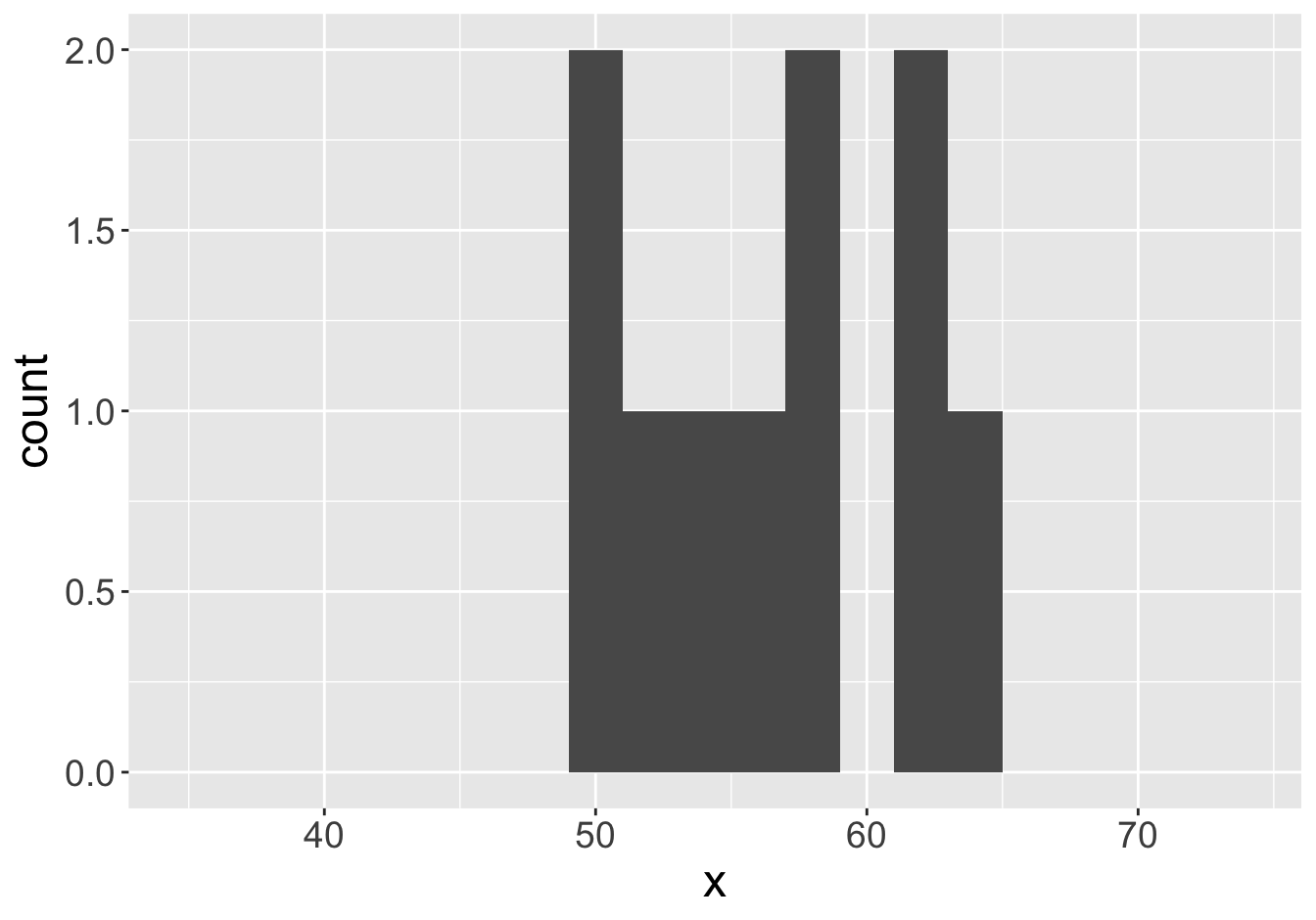
Example - Means (Sample Size 2)

Mean: 55.06
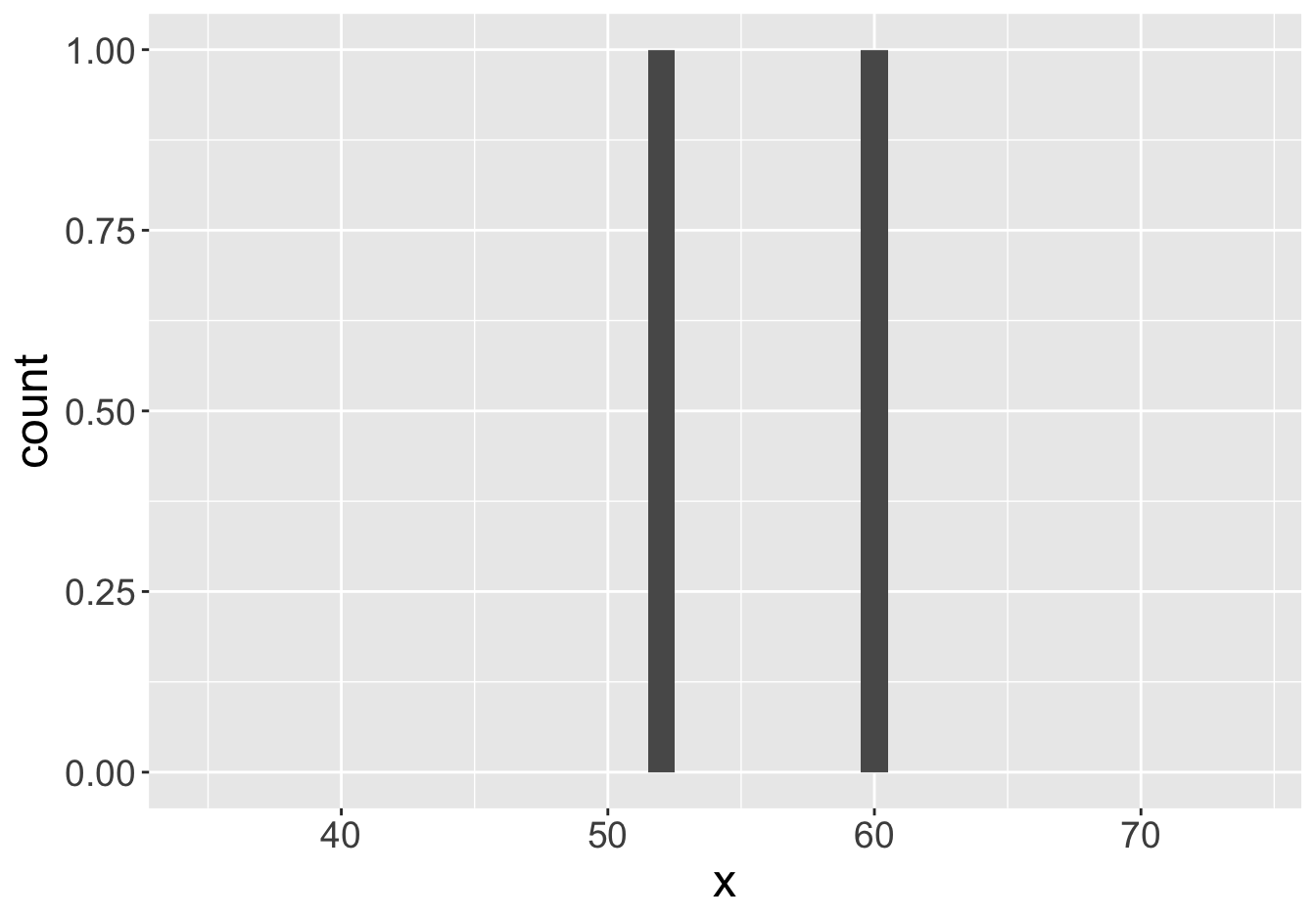
Mean: 55.9
Example - Means (Sample Size 2)

Mean: 55.06
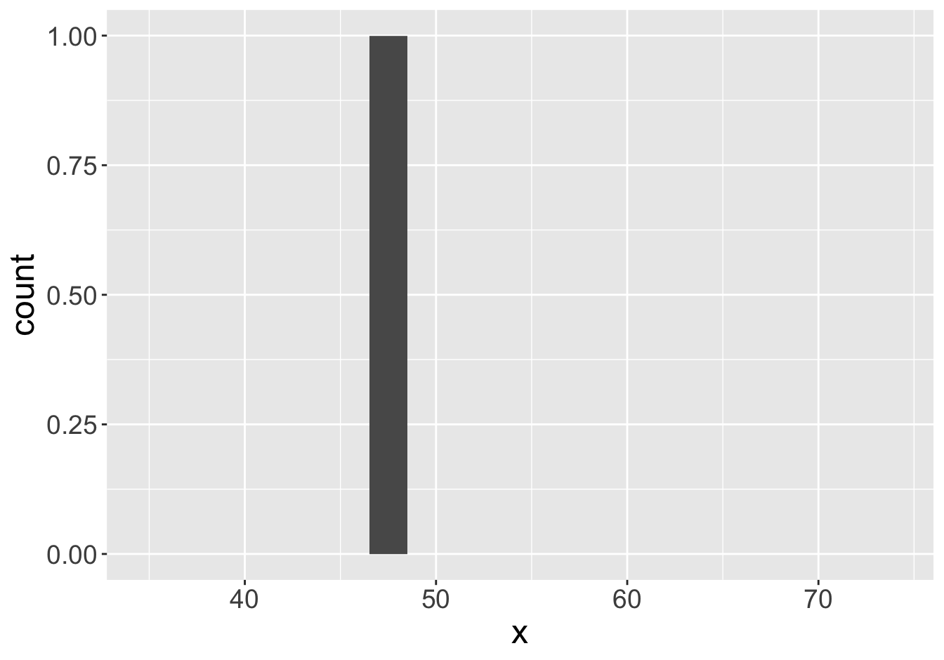
Mean: 47.8
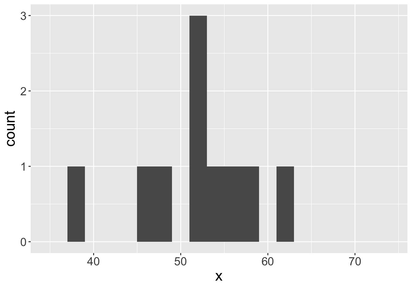
Example - Means (Sample Size 2)

Mean: 55.06
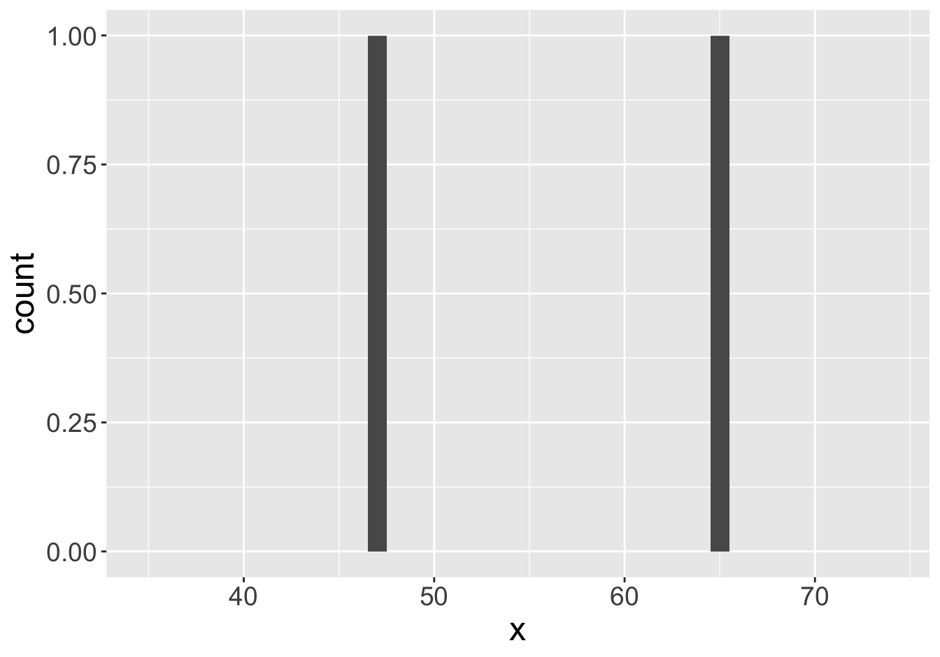
Mean: 56.08
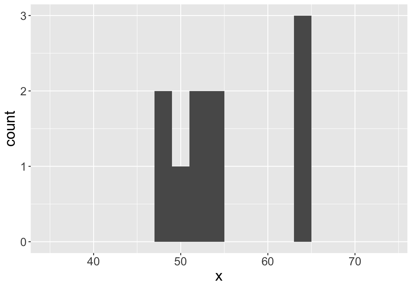
Example - Means (Sample Size 2)

Mean: 55.06
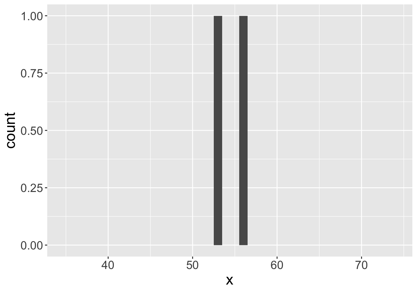
Mean: 54.38
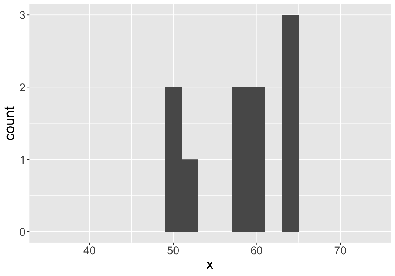
Example - Means (Sample Size 2)

Mean: 55.06
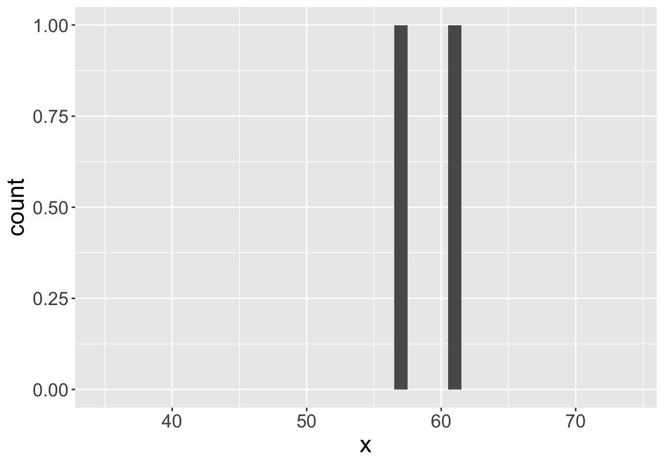
Mean: 59.24
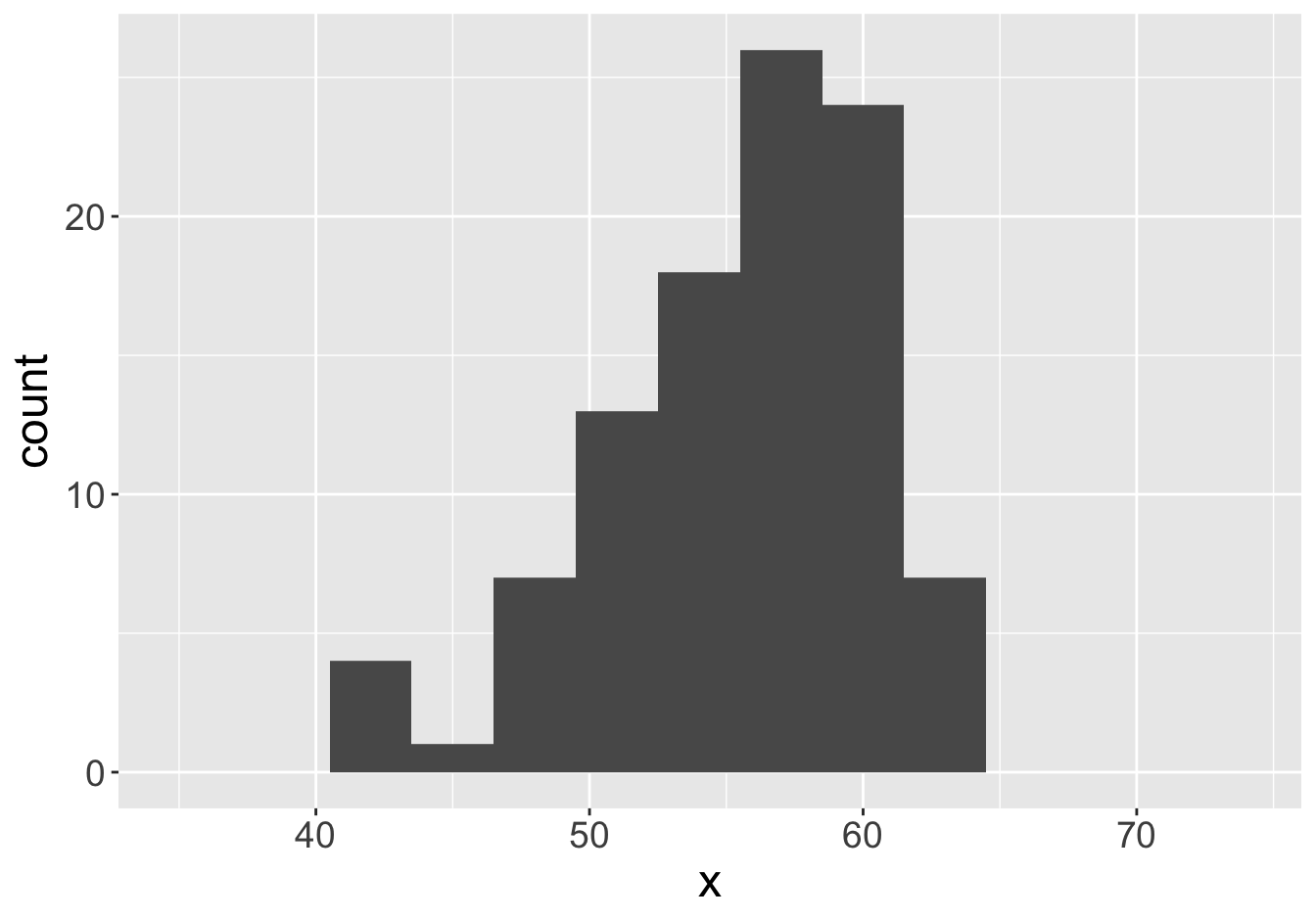
Example - Means (Sample Size 10)

Mean: 55.06
Mean: 53.29
Example - Means (Sample Size 10)

Mean: 55.06
Mean: 51.59
Example - Means (Sample Size 10)

Mean: 55.06
Mean: 55.24
Example - Means (Sample Size 10)

Mean: 55.06
Mean: 57.99
Example - Means (Sample Size 10)

Mean: 55.06
Mean: 56.54
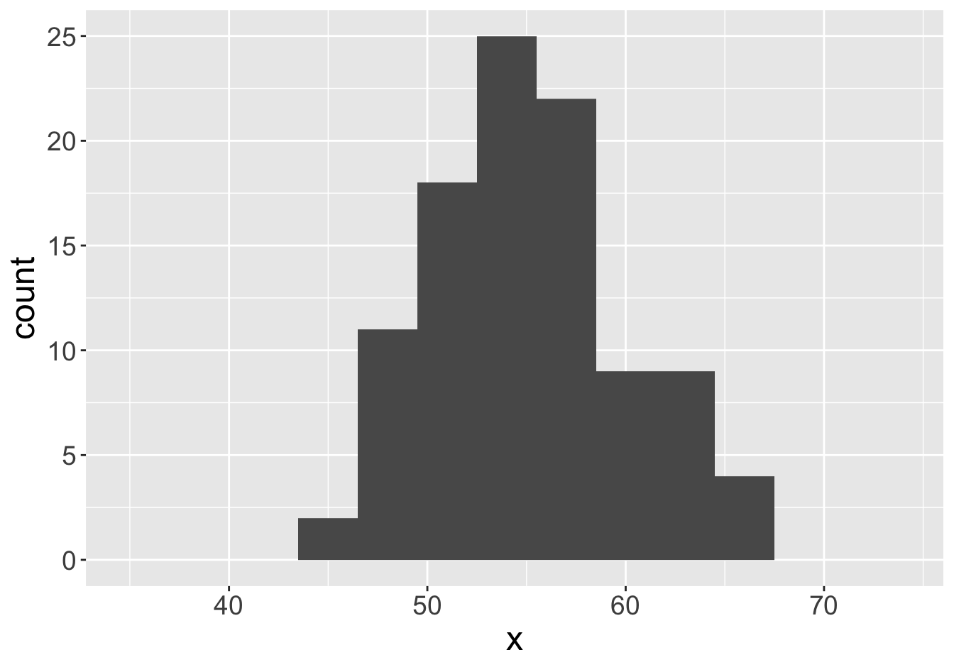
Example - Means (Sample Size 100)

Mean: 55.06
Mean: 55.55
Example - Means (Sample Size 100)

Mean: 55.06
Mean: 54.84
Example - Means (Sample Size 100)

Mean: 55.06
Mean: 54.98
Example - Means (Sample Size 100)

Mean: 55.06
Mean: 54.58
Example - Means (Sample Size 100)
Mean: 55.06
Mean: 55.57
Example - Means (Sample Size 100)

Mean: 55.06
Mean: 55.12
Example - Means (Sample Size 100)

Mean: 55.06
Mean: 55.29
Example - Means (Sample Size 1000)

Mean: 55.06
Mean: 55.07
Example - Means (Sample Size 1000)

Mean: 55.06
Mean: 55.06
Example - Means (Sample Size 1000)

Mean: 55.06
Mean: 55.05
Example - Means
How confident would you feel stating that the population mean is equal to any of these values?
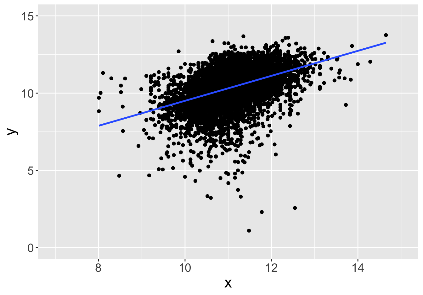
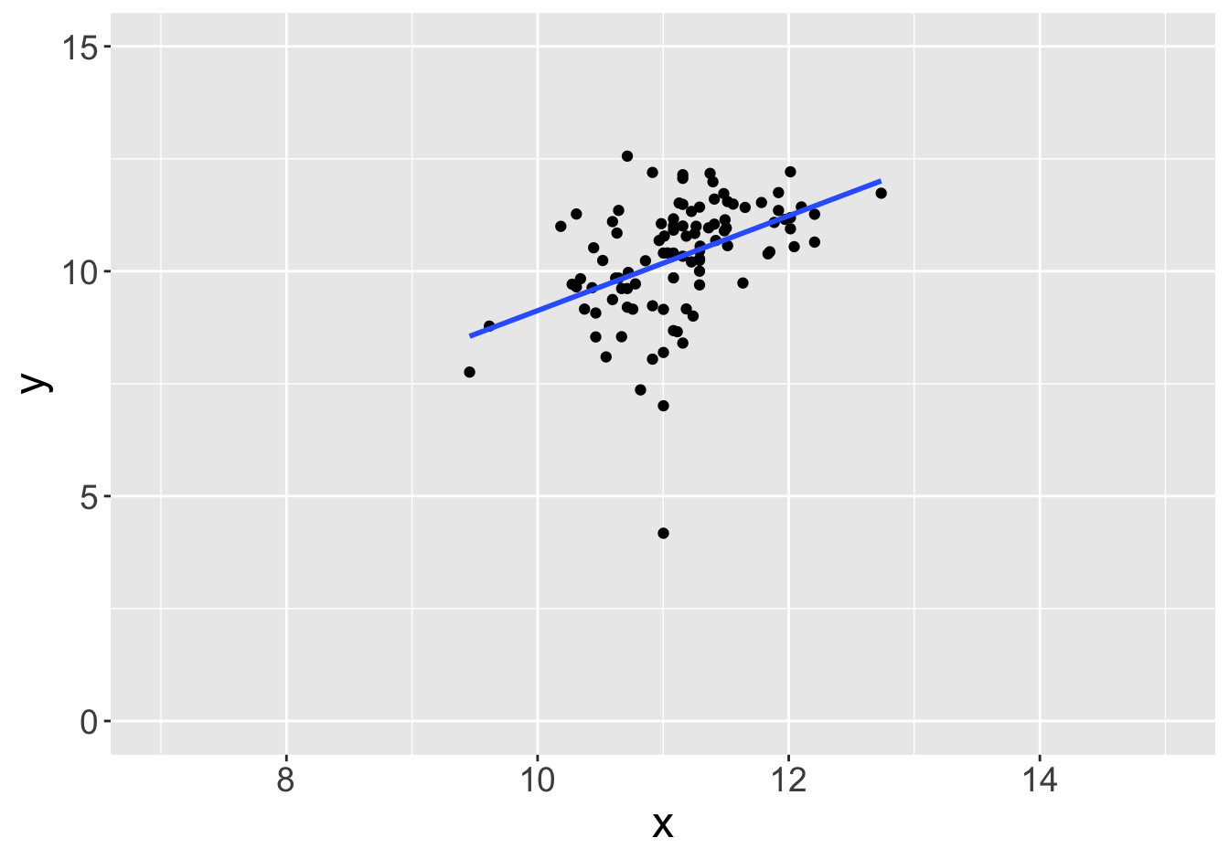
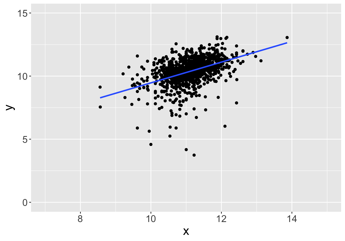
Example - Slopes
Suppose this scatter plot represents some values \(x, y\) in a population of 10,000:
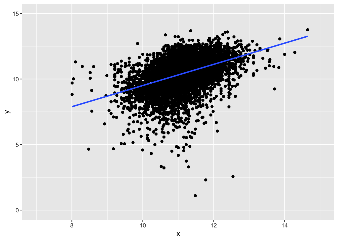
Slope: 0.81
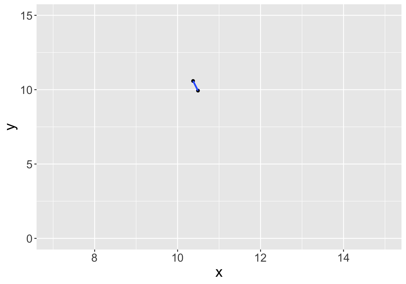
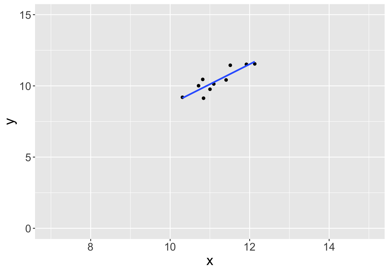
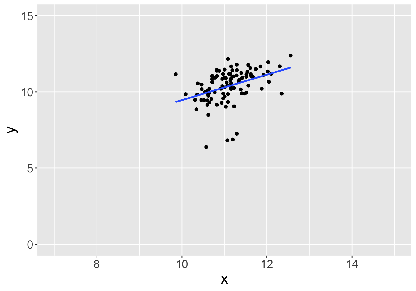
Example - Slopes (Sample Size 2)

Slope: 0.81
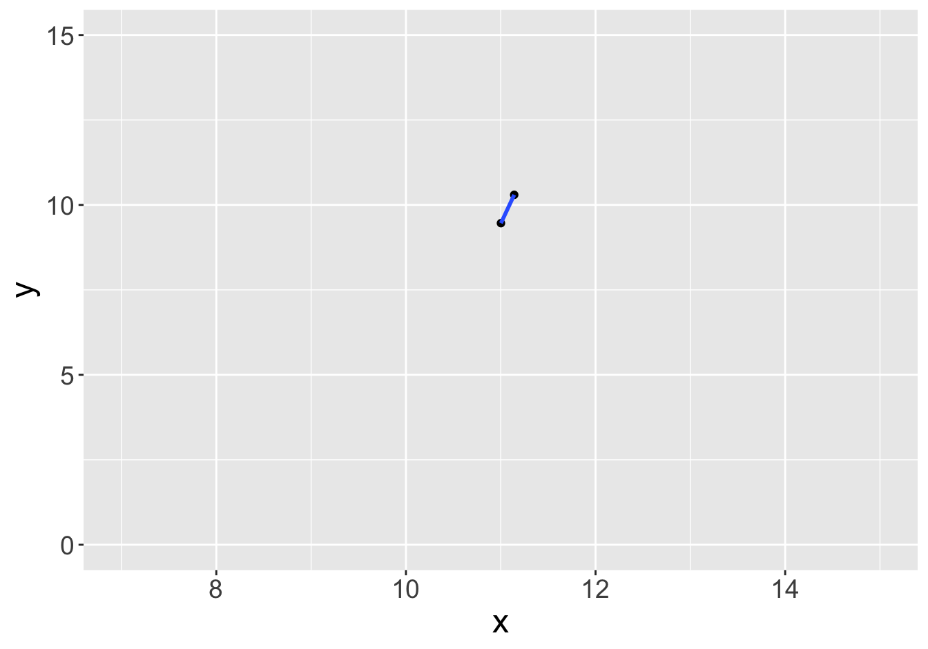
Slope: 5.97
Example - Slopes (Sample Size 2)

Slope: 0.81
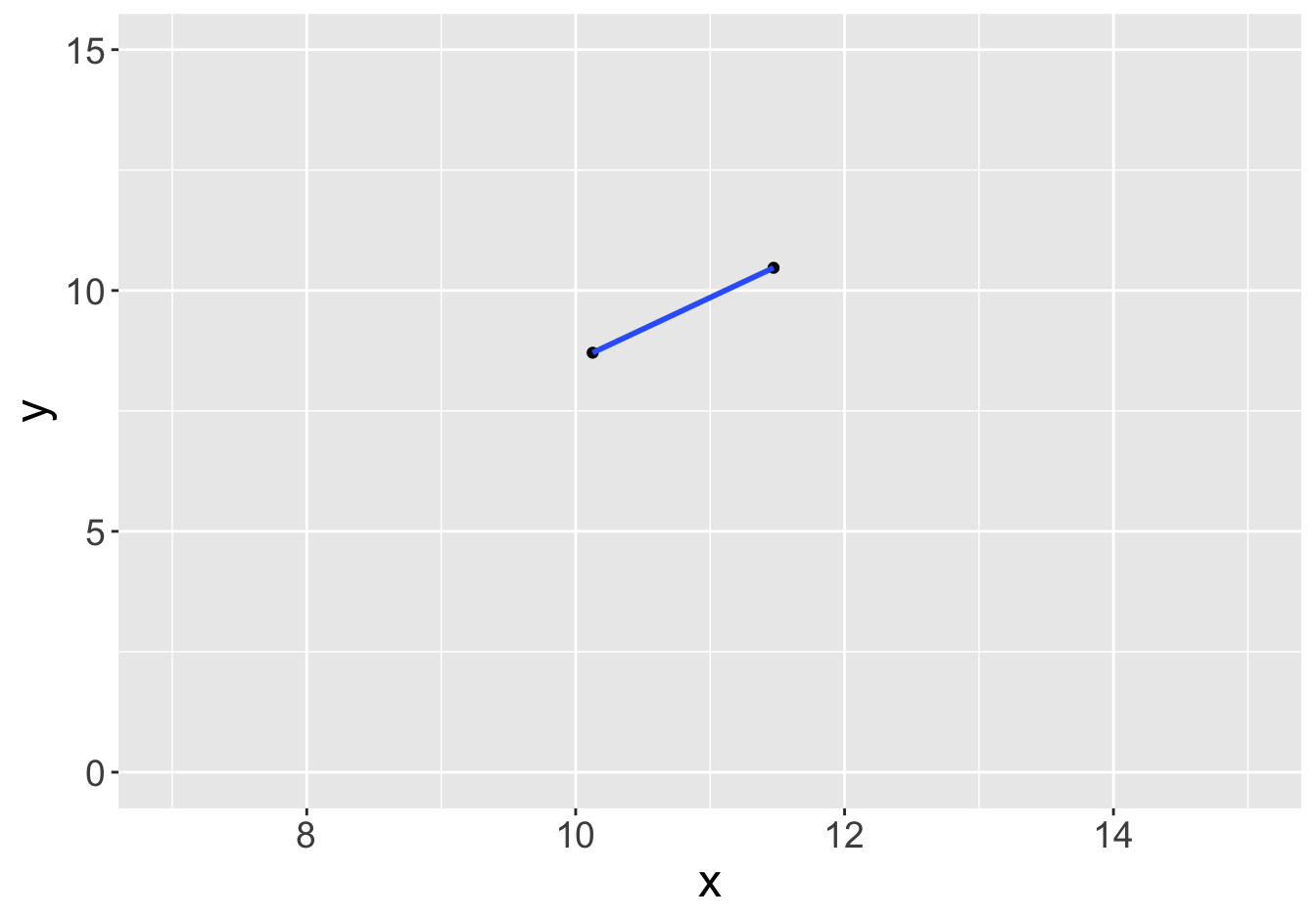
Slope: 1.31
Example - Slopes (Sample Size 2)

Slope: 0.81
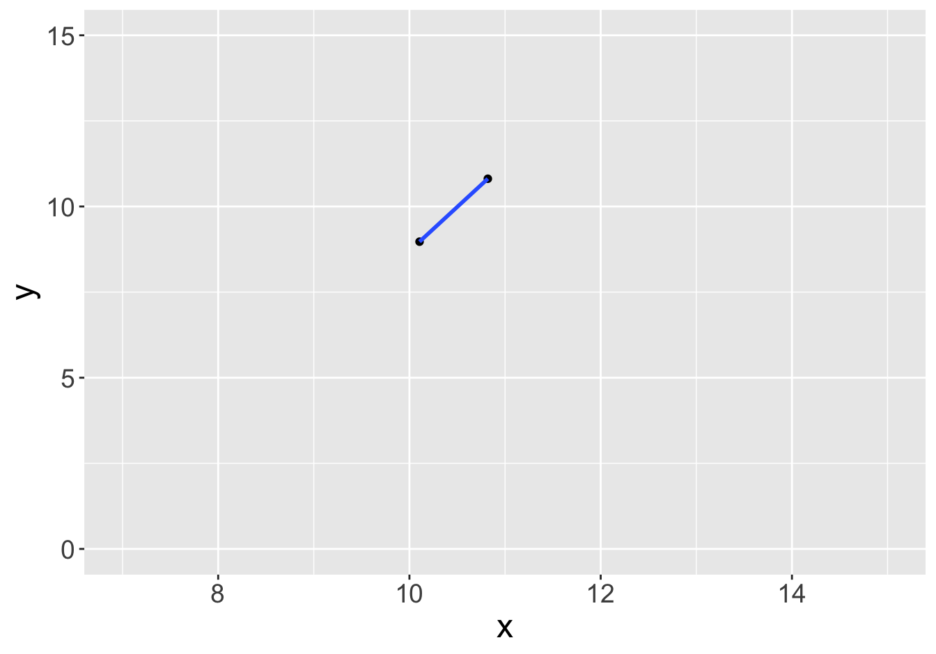
Slope: 2.57
Example - Slopes (Sample Size 2)

Slope: 0.81
Slope: -5.51
Example - Slopes (Sample Size 10)

Slope: 0.81
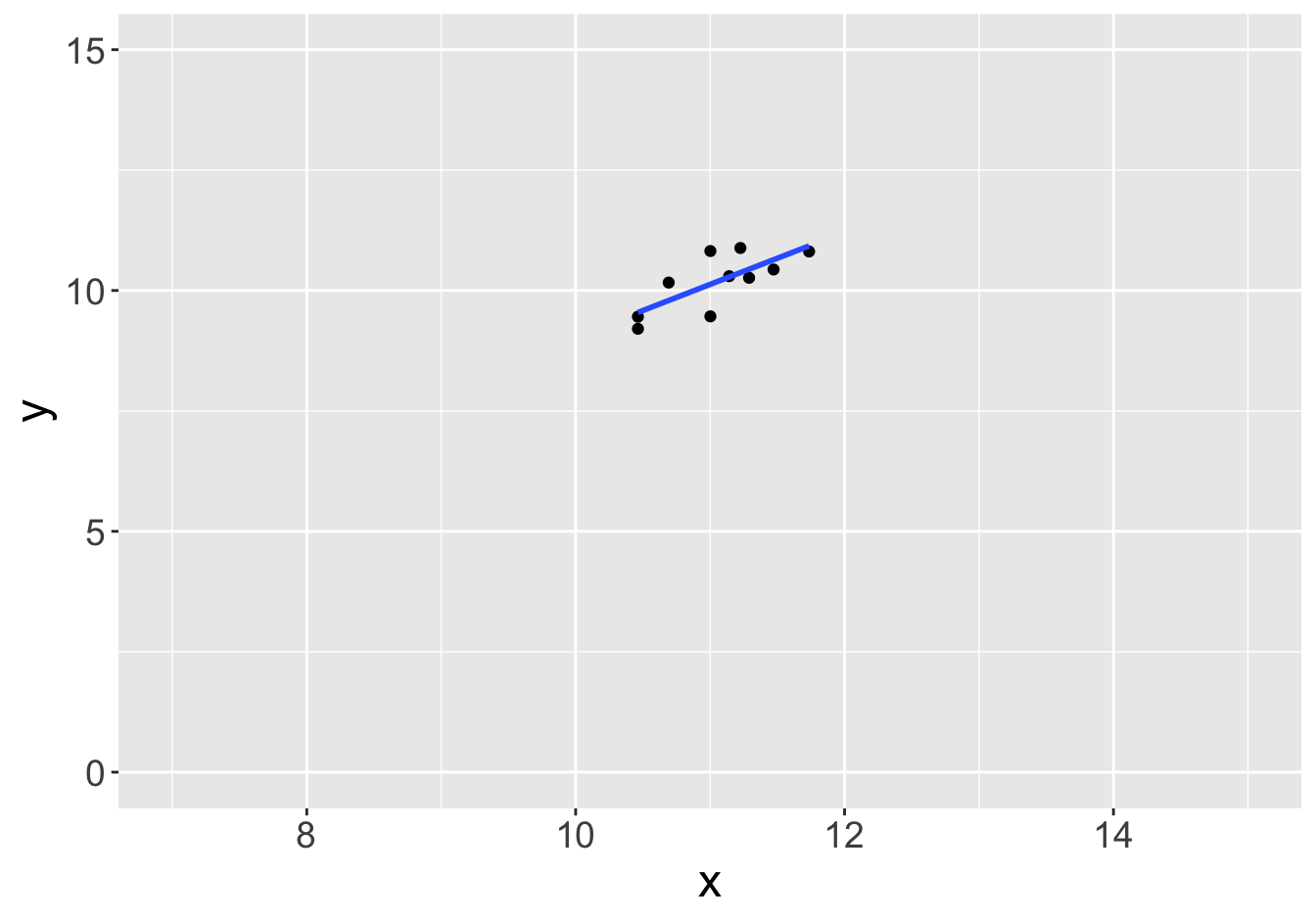
Slope: 1.08
Example - Slopes (Sample Size 10)
Slope: 0.81
Slope: 1.01
Example - Slopes (Sample Size 10)

Slope: 0.81
Slope: 1.41
Example - Slopes (Sample Size 10)

Slope: 0.81
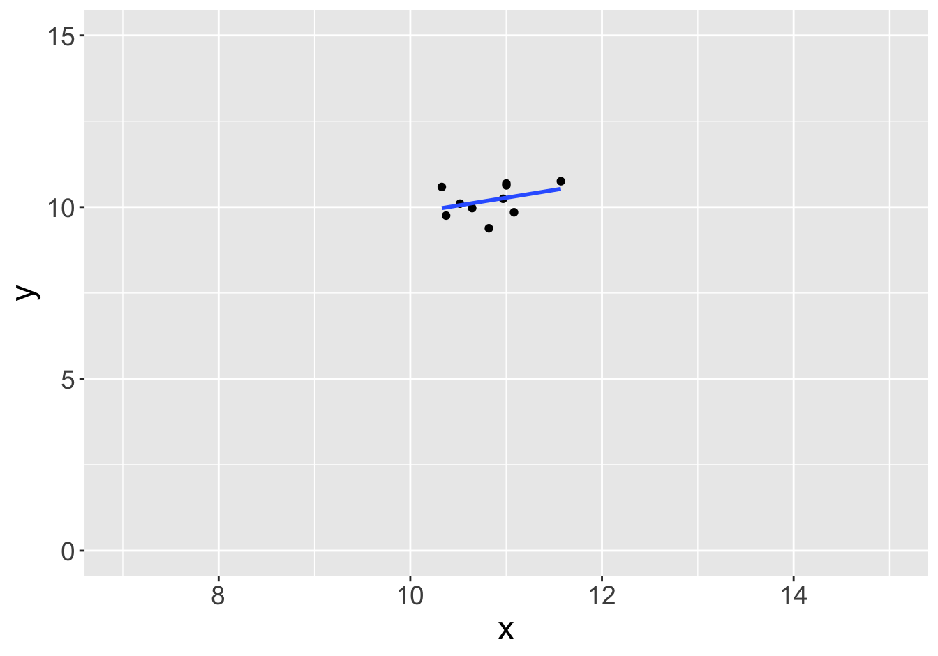
Slope: 0.45
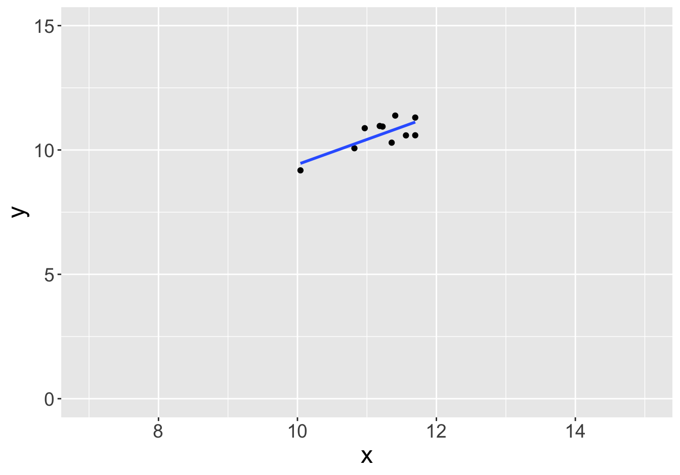
Example - Slopes (Sample Size 100)

Slope: 0.81
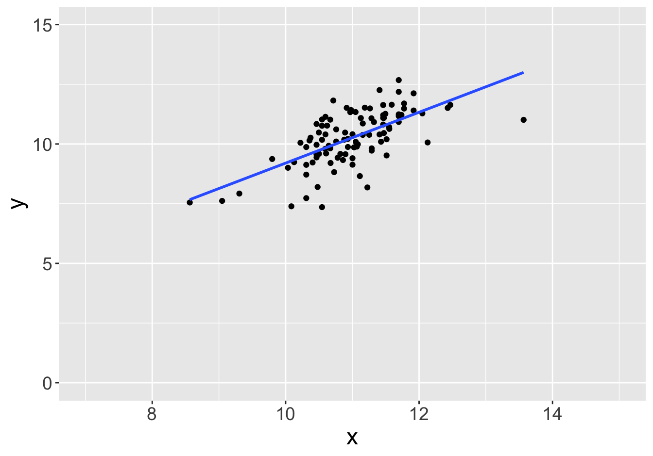
Slope: 1.06
Example - Slopes (Sample Size 100)

Slope: 0.81
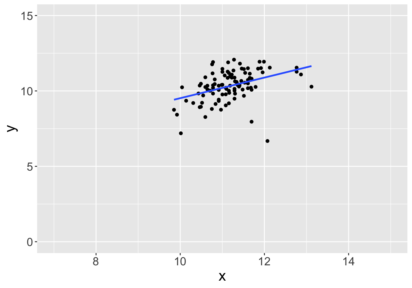
Slope: 0.68
Example - Slopes (Sample Size 100)

Slope: 0.81
Slope: 1.05
Example - Slopes (Sample Size 100)

Slope: 0.81
Slope: 0.84
Example - Slopes (Sample Size 100)

Slope: 0.81

Slope: 0.64
Example - Slopes (Sample Size 1000)

Slope: 0.81
Slope: 0.77
Example - Slopes (Sample Size 1000)

Slope: 0.81
Slope: 0.72
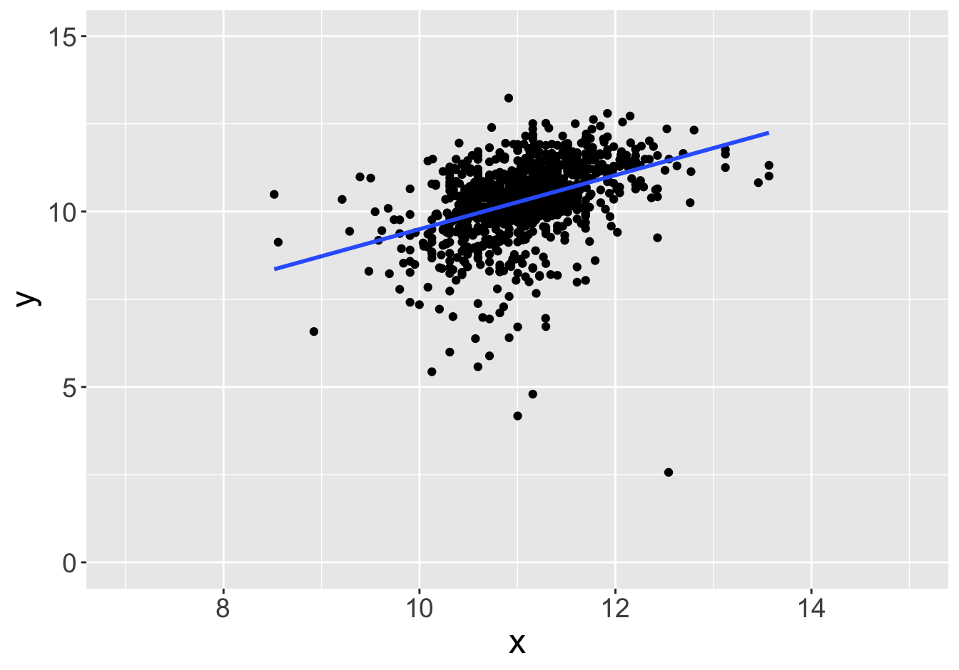
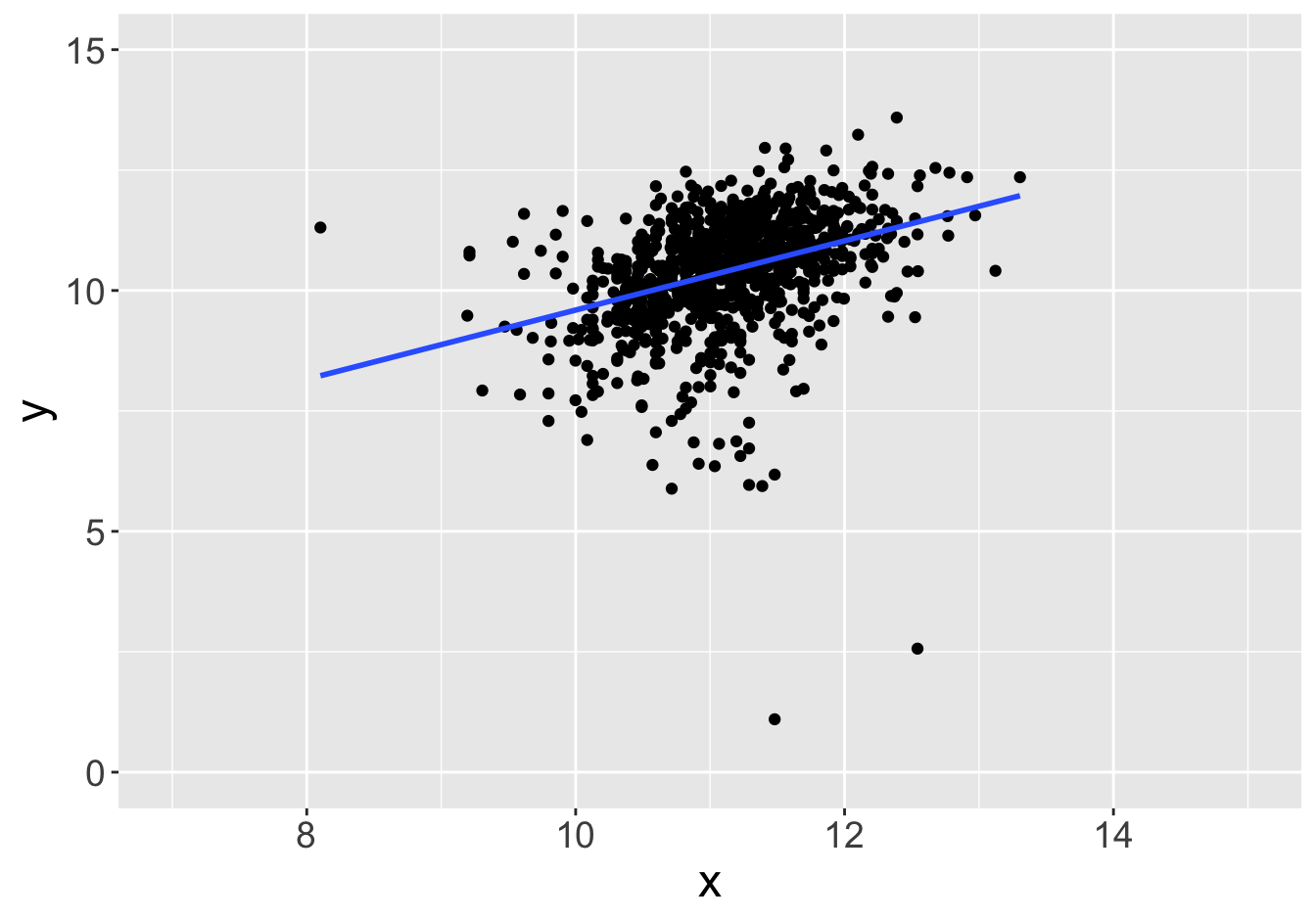
Example - Slopes (Sample Size 1000)

Slope: 0.81
Slope: 0.82
Example - Slopes
How confident would you feel stating that the population slope is equal to any of these values?s
The Vision
How can we give a range of reasonable values for the population data using the sample data we have??
Idea: use the sample to take more samples???
Method: bootstrapping!
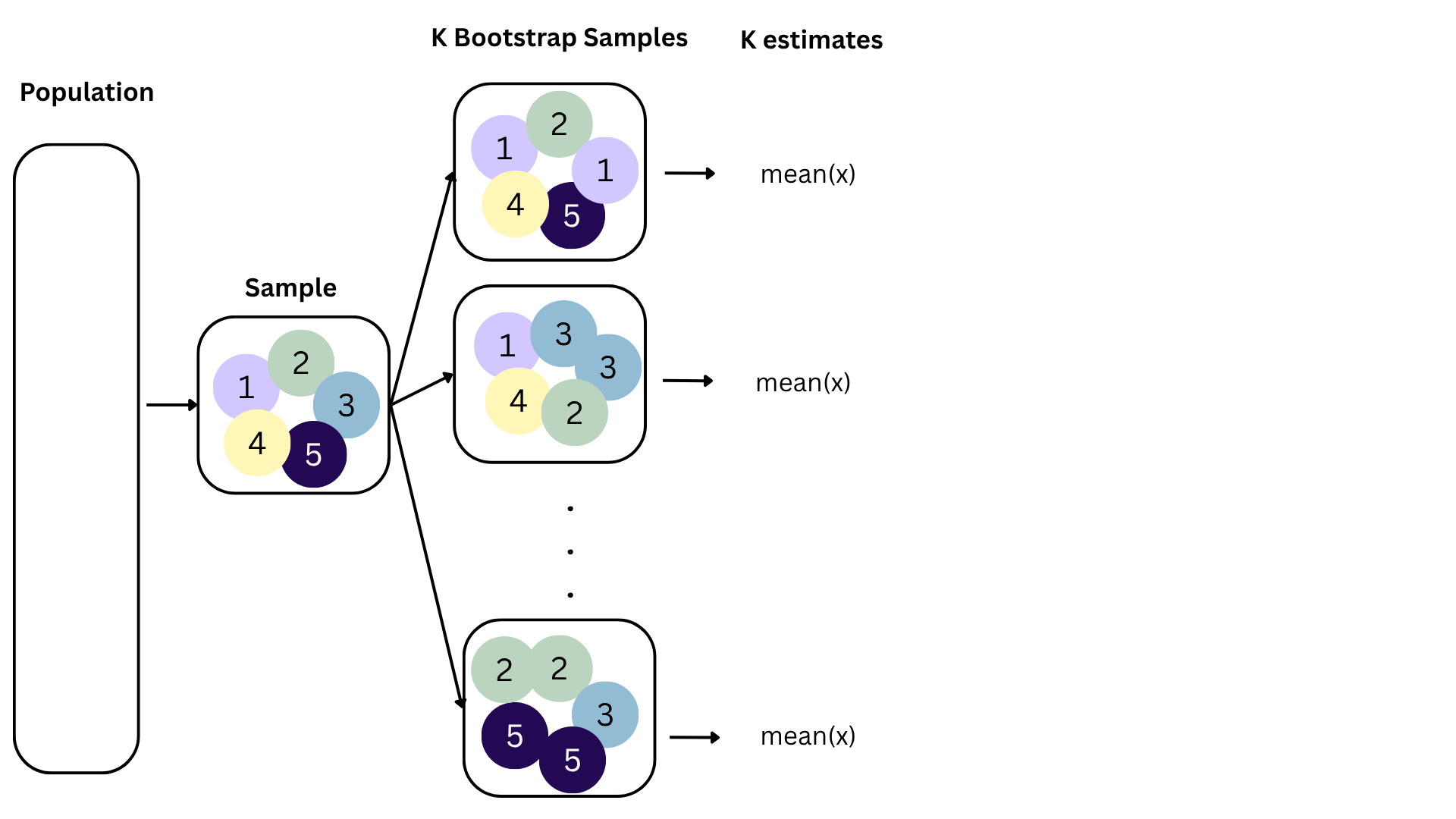
Bootstrapping
Bootstrapping
Bootstrapping
Bootstrapping
Bootstrapping
Bootstrapping
Bootstrapping
Today’s Goal
Find range of plausible values for a slope using bootstrap confidence intervals.
Data: Houses in Duke Forest
- Data on houses that were sold in the Duke Forest neighborhood of Durham, NC around November 2020
- Pulled from Zillow
- Source:
openintro::duke_forest
. . .
Goal: Use the area (in square feet) to understand variability in the price of houses in Duke Forest.
Exploratory data analysis
Code
ggplot(duke_forest, aes(x = area, y = price)) +
  geom_point(alpha = 0.7) +
  labs(
    x = "Area (square feet)",
    y = "Sale price (USD)",
    title = "Price and area of houses in Duke Forest"
  ) +
scale_y_continuous(labels = label_dollar()) 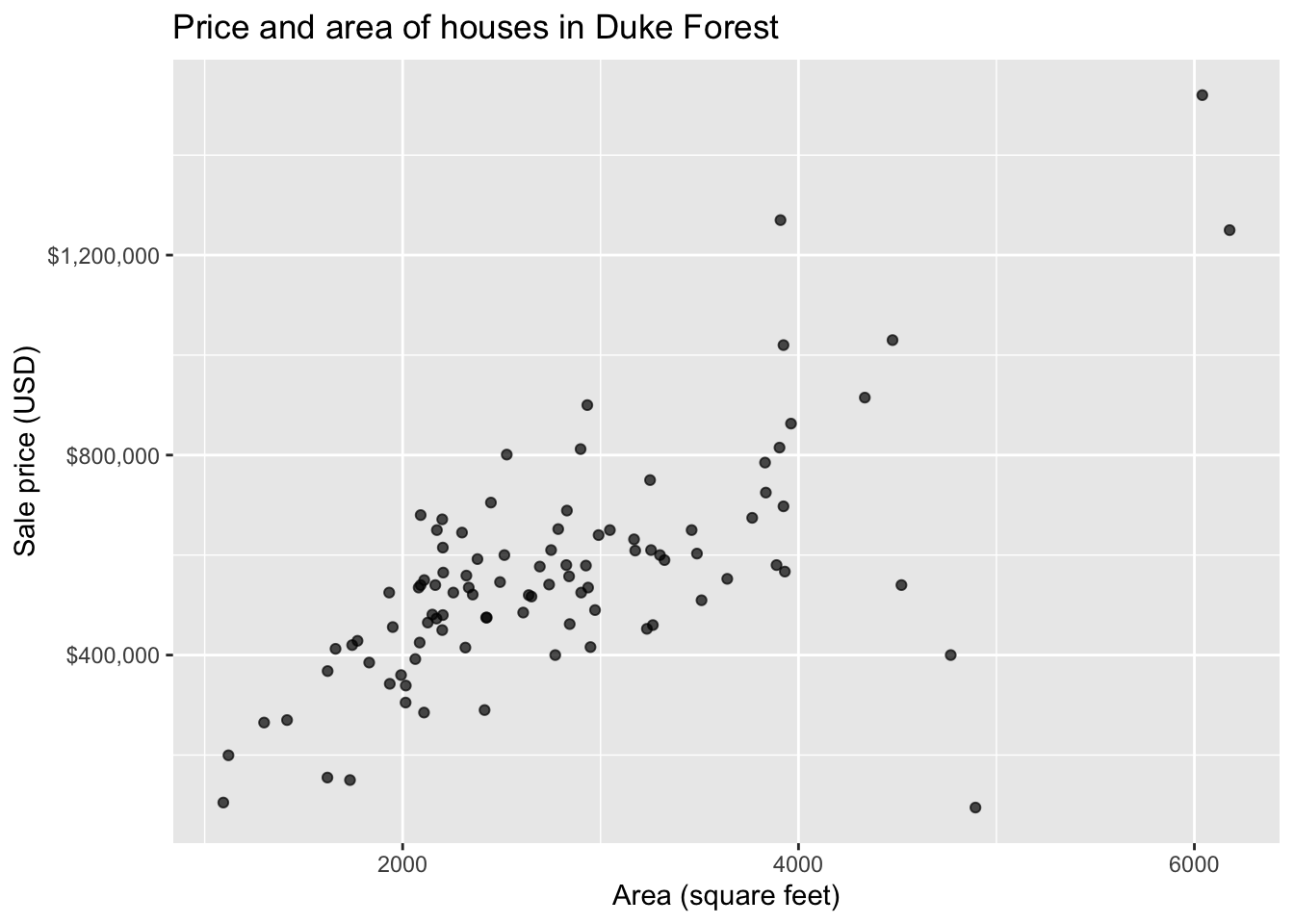
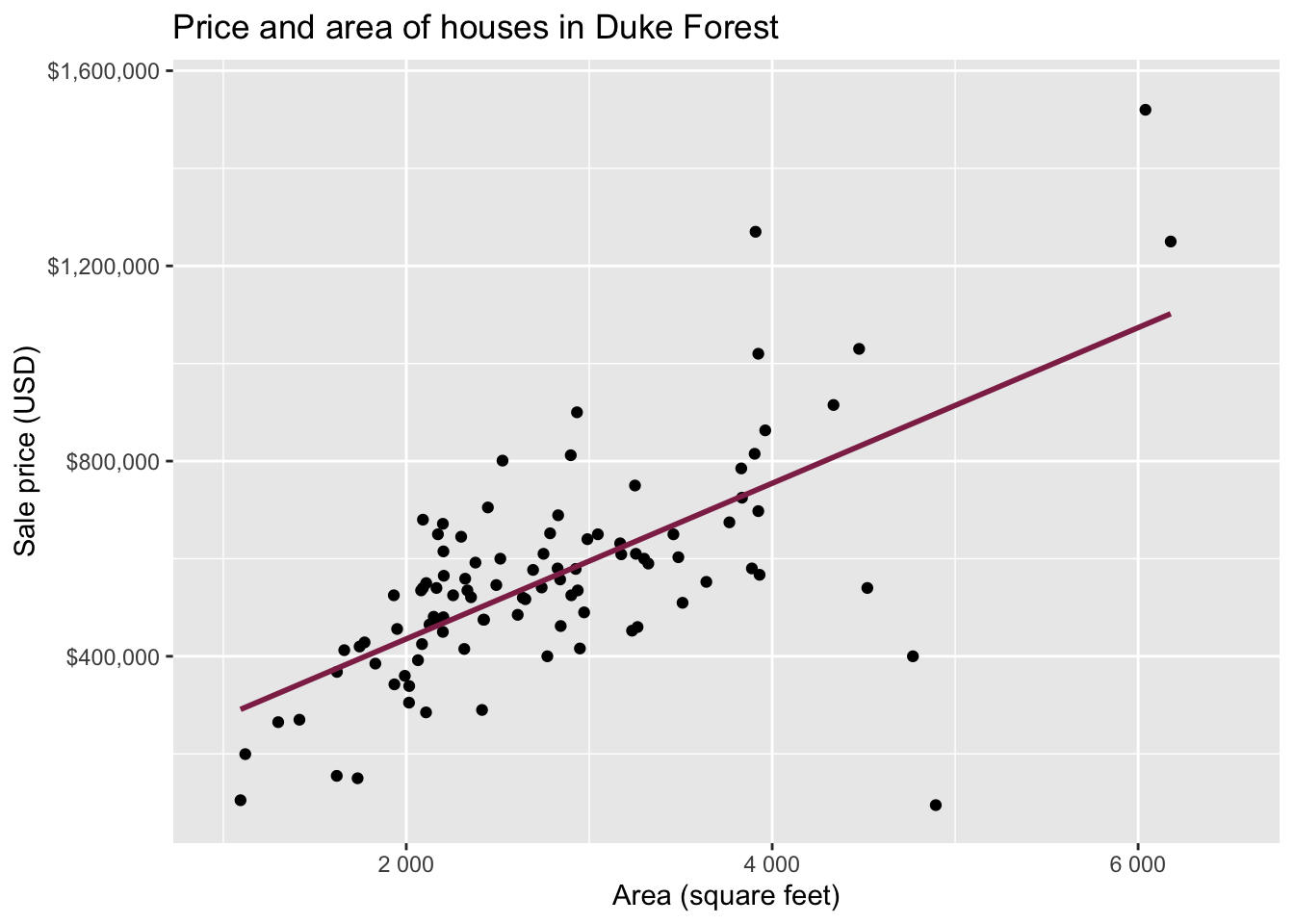
Modeling
df_fit <- linear_reg() |>
  fit(price ~ area, data = duke_forest)

tidy(df_fit)
# A tibble: 2 × 5
term estimate std.error statistic p.value
<chr> <dbl> <dbl> <dbl> <dbl>
1 (Intercept) 116652. 53302. 2.19 3.11e- 2
2 area 159. 18.2 8.78 6.29e-14. . .
Intercept: Duke Forest houses that are 0 square feet are expected to sell, for $116,652, on average.
Slope: For each additional square foot, we expect the sale price of Duke Forest houses to be higher by $159, on average.
From sample to population
For each additional square foot, we expect the sale price of Duke Forest houses to be higher by $159, on average.
- This estimate is valid for the single sample of 98 houses.
- But what if we’re not interested quantifying the relationship between the size and price of a house in this single sample?
- What if we want to say something about the relationship between these variables for all houses in Duke Forest?
Inference for simple linear regression
Calculate a confidence interval for the slope, \(\beta_1\) (today)
Conduct a hypothesis test for the slope,\(\beta_1\) (next week)
Confidence interval for the slope
Confidence interval
- A plausible range of values for a population parameter is called a confidence interval
- Using only a single point estimate is like fishing in a murky lake with a spear. Using a confidence interval is like fishing with a net.
- We can throw a spear where we saw a fish but we will probably miss. If we toss a net in that area, we have a good chance of catching the fish.
- If we report a point estimate, we probably will not hit the exact population parameter. If we report a range of plausible values we have a good shot at capturing the parameter
Confidence interval for the slope
A confidence interval will allow us to make a statement like “For each additional square foot, the model predicts the sale price of Duke Forest houses to be higher, on average, by $159, plus or minus X dollars.”
. . .
Should X be $10? $100? $1000?
If we were to take another sample of 98 would we expect the slope calculated based on that sample to be exactly $159? Off by $10? $100? $1000?
. . .
- The answer depends on how variable (from one sample to another sample) the sample statistic (the slope) is
. . .
- We need a way to quantify the variability of the sample statistic
Quantify the variability of the slope
- Two approaches:
- Via simulation (what we’ll do in this course)
- Via mathematical models (what you can learn about in future courses)
Quantify the variability of the slope
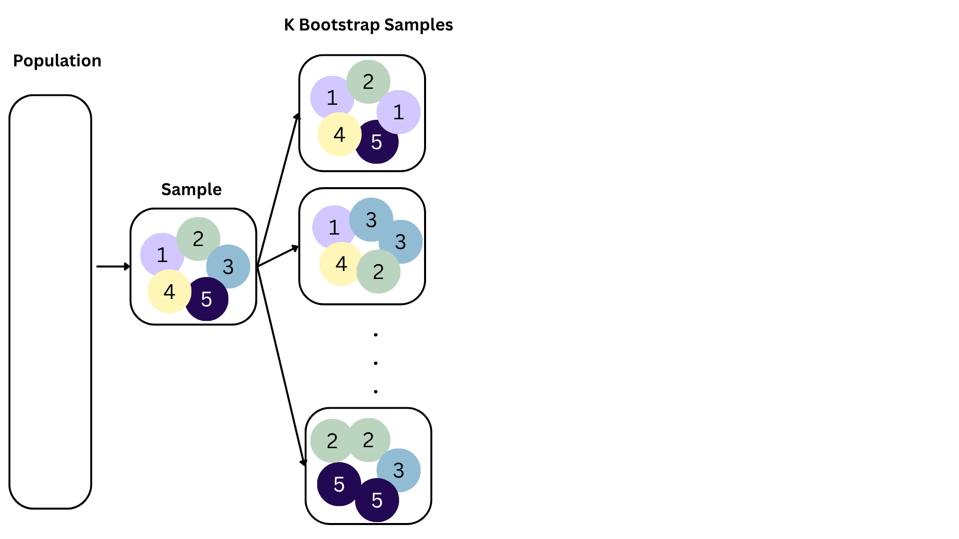
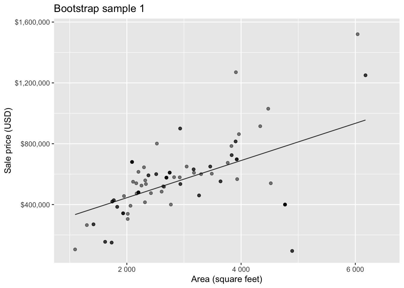
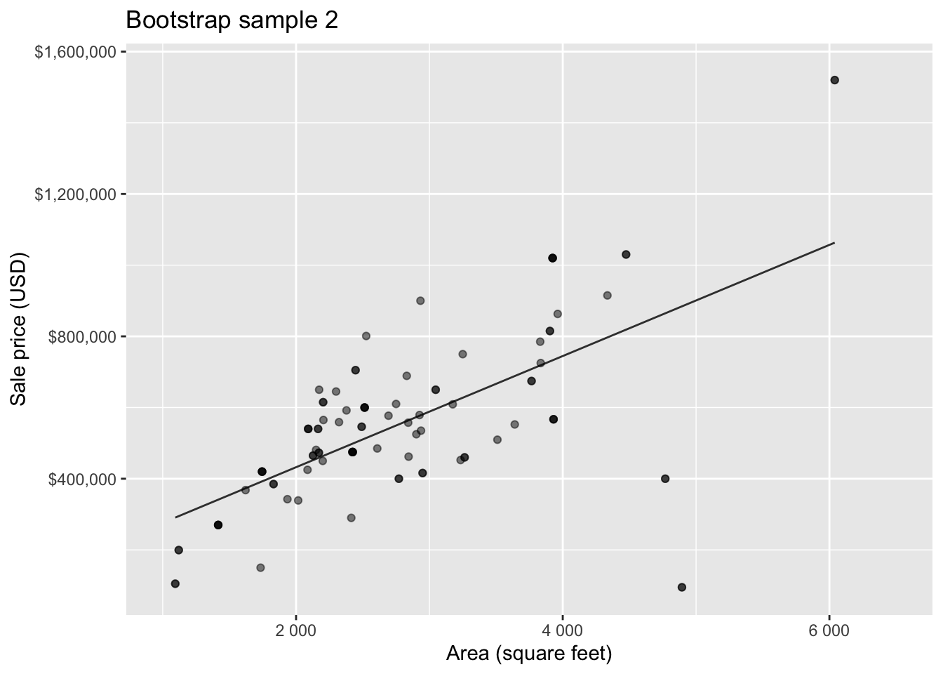
Bootstrapping to quantify the variability of the slope for the purpose of estimation:
- Bootstrap new samples from the original sample
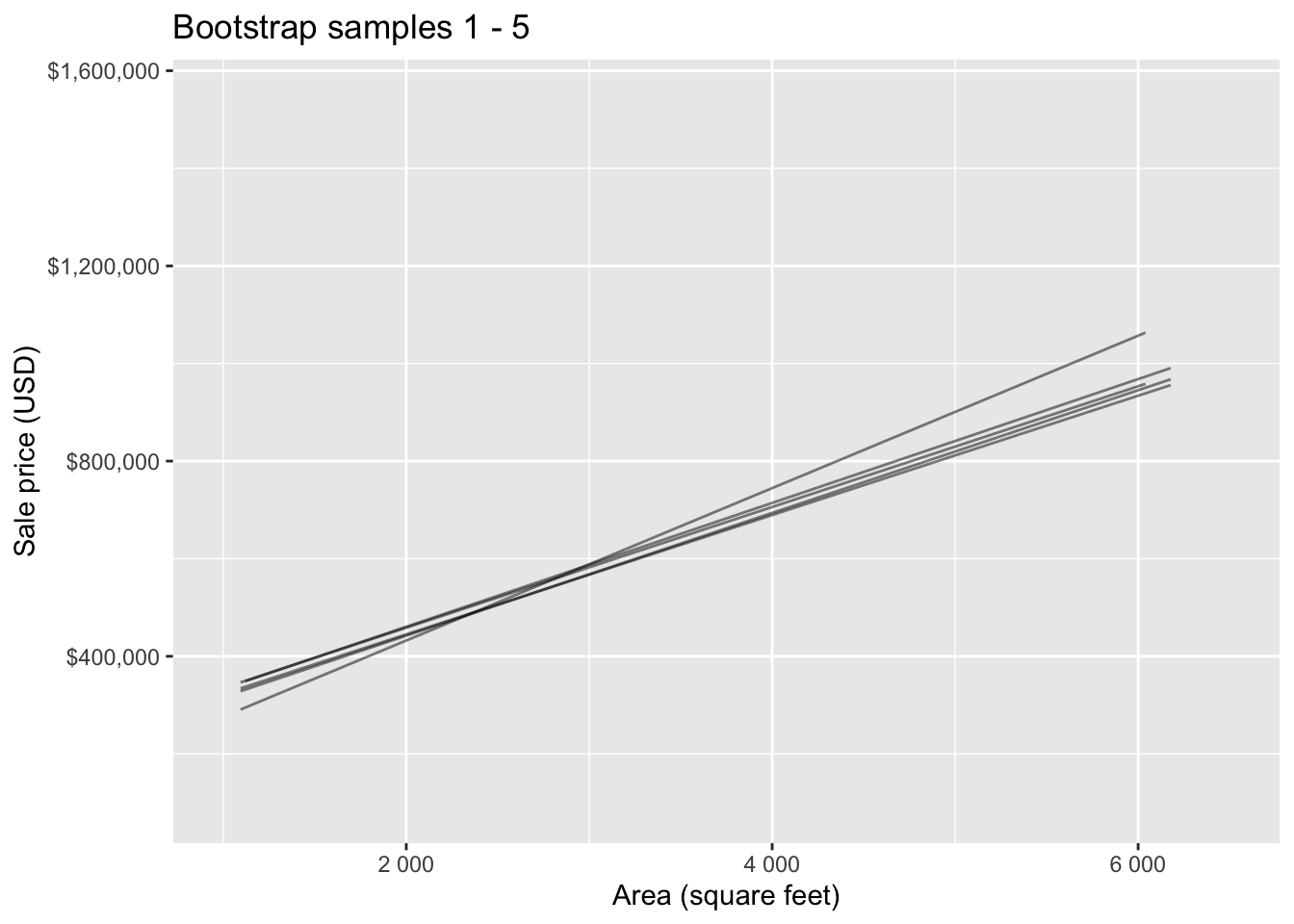
- Fit models to each of the samples and estimate the slope
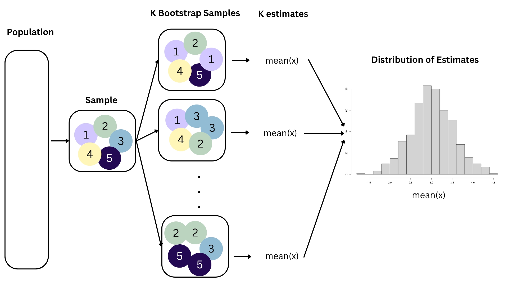
- Use features of the distribution of the bootstrapped slopes to construct a confidence interval
Bootstrap sample 1

Bootstrap sample 2
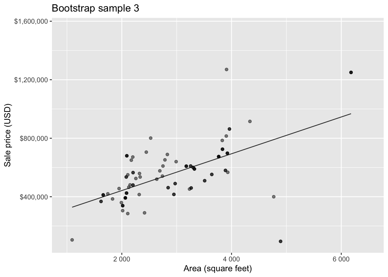
Bootstrap sample 3

Bootstrap sample 4


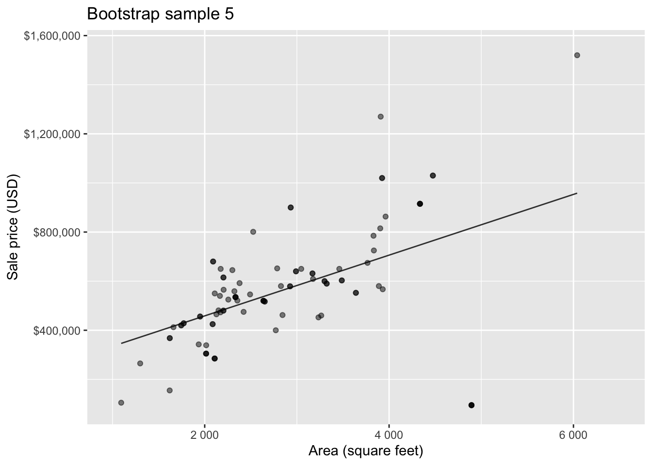
Bootstrap sample 5

. . .
so on and so forth…
Bootstrap samples 1 - 5

Bootstrap samples 1 - 100

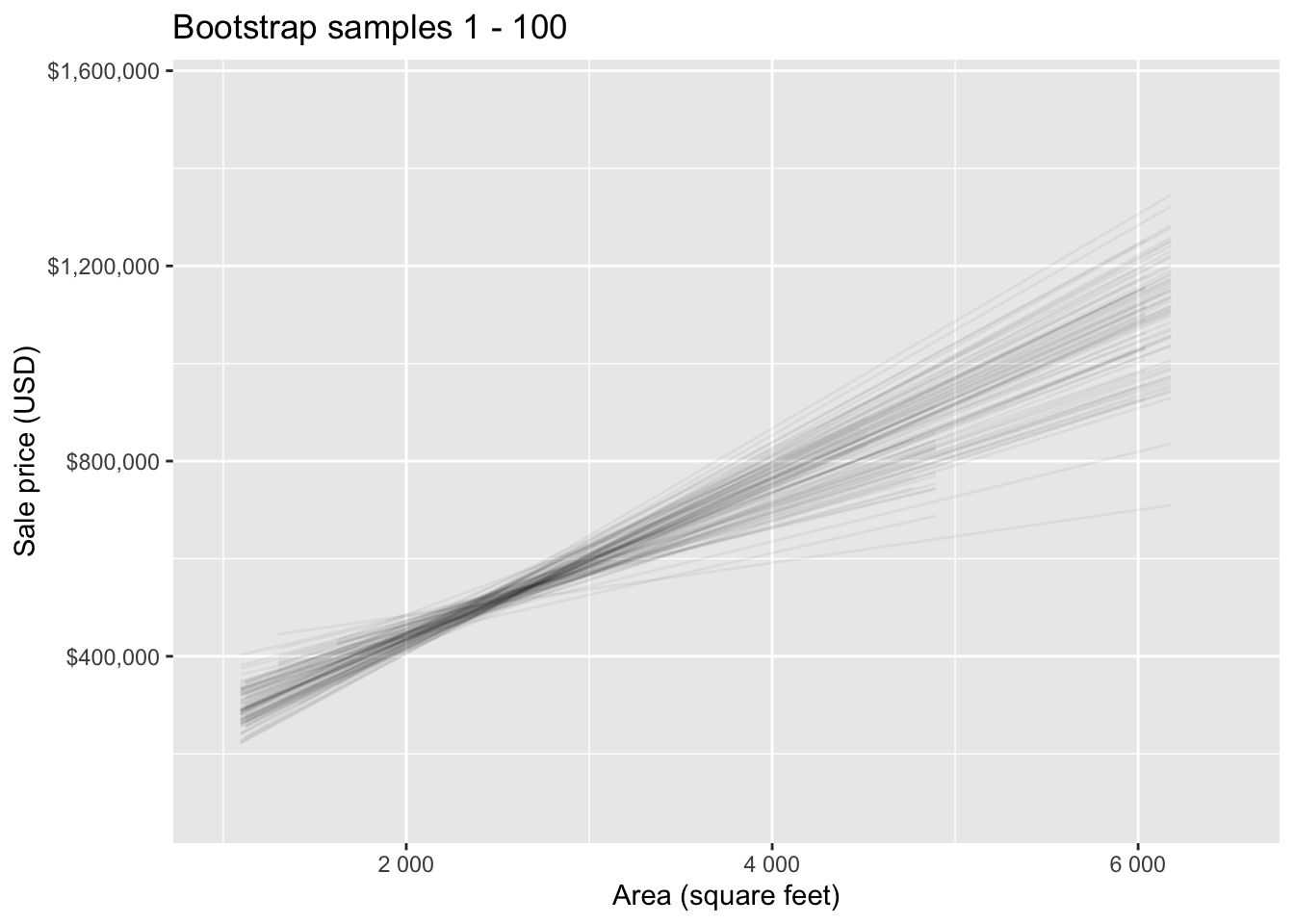
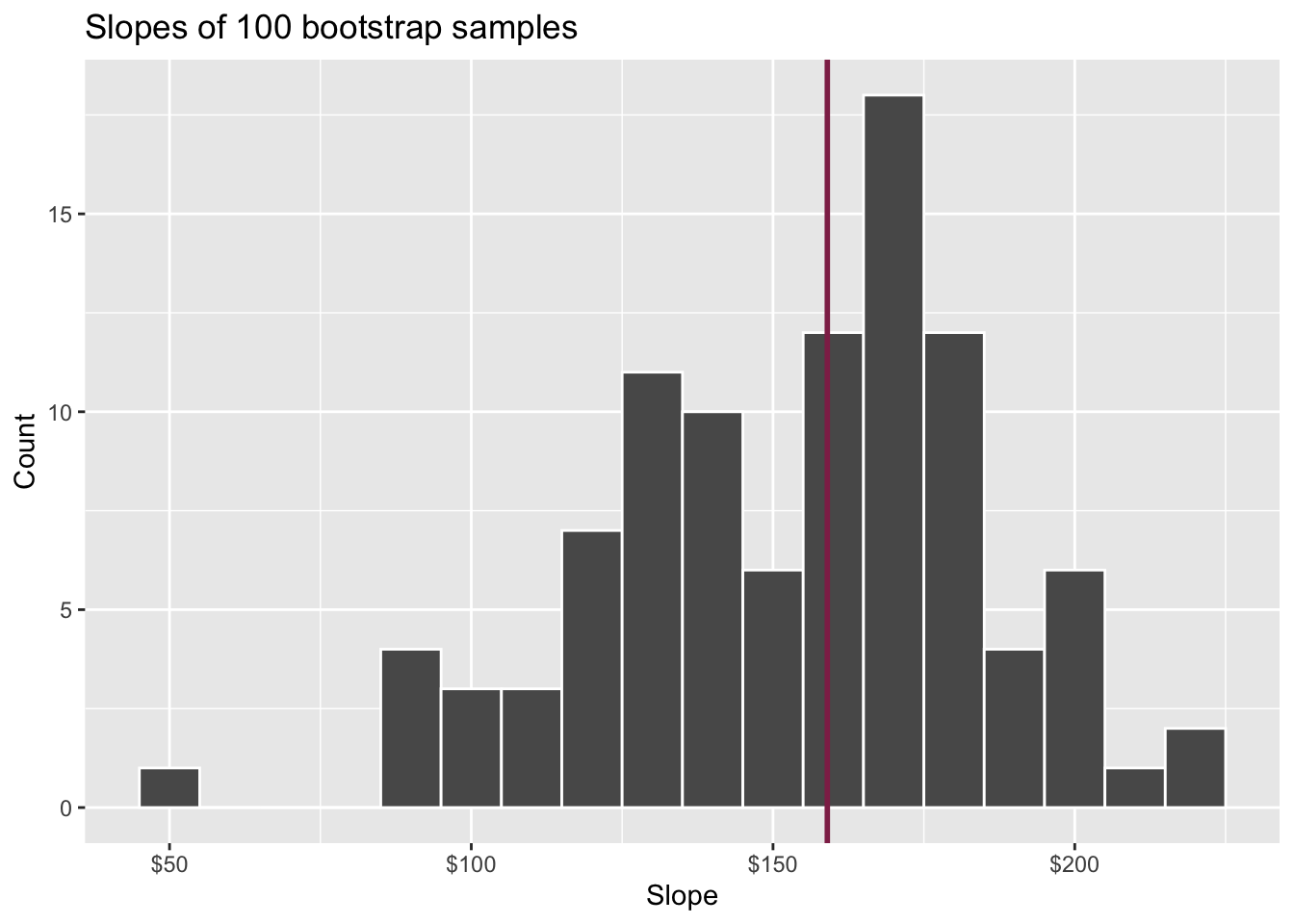
Slopes of bootstrap samples
Fill in the blank: For each additional square foot, the model predicts the sale price of Duke Forest houses to be higher, on average, by $159, plus or minus ___ dollars.
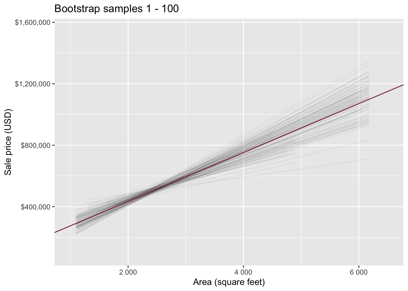
Slopes of bootstrap samples
Fill in the blank: For each additional square foot, we expect the sale price of Duke Forest houses to be higher, on average, by $159, plus or minus ___ dollars.

Confidence level
How confident are you that the true slope is between $0 and $250? How about $150 and $170? How about $90 and $210?
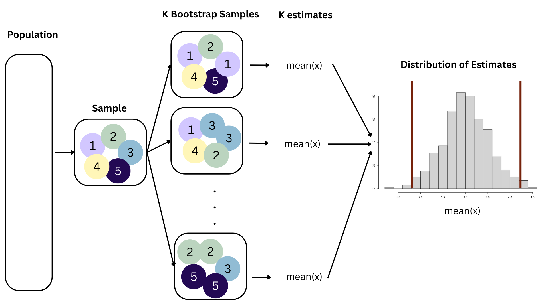
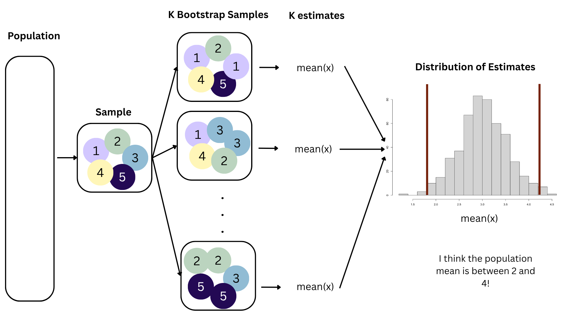
95% confidence interval
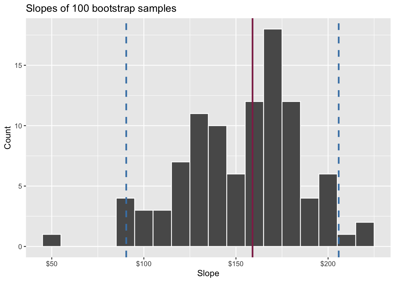
- A 95% confidence interval is bounded by the middle 95% of the bootstrap distribution
- We are 95% confident that for each additional square foot, the model predicts the sale price of Duke Forest houses to be higher, on average, by $90.43 to $205.77.
Application exercise
Calculate observed fit
Calculate the observed slope:
observed_fit <- duke_forest |>
  specify(price ~ area) |>
  fit()

observed_fit
# A tibble: 2 × 2
term estimate
<chr> <dbl>
1 intercept 116652.
2 area 159.Take bootstrap samples
Take 100 bootstrap samples and fit models to each one:
set.seed(1234)
n = 100

boot_fits <- duke_forest |>
  specify(price ~ area) |>
  generate(reps = n, type = "bootstrap") |>
  fit()

boot_fits
# A tibble: 200 × 3
# Groups: replicate [100]
replicate term estimate
<int> <chr> <dbl>
1 1 intercept 177388.
2 1 area 125.
3 2 intercept 161078.
4 2 area 150.
5 3 intercept 202354.
6 3 area 118.
7 4 intercept 120750.
8 4 area 162.
9 5 intercept 52127.
10 5 area 180.
# ℹ 190 more rowsExamine bootstrap samples
boot_fits |>
  filter(term == "area") |>
  ggplot(aes(x = estimate)) +
  geom_histogram()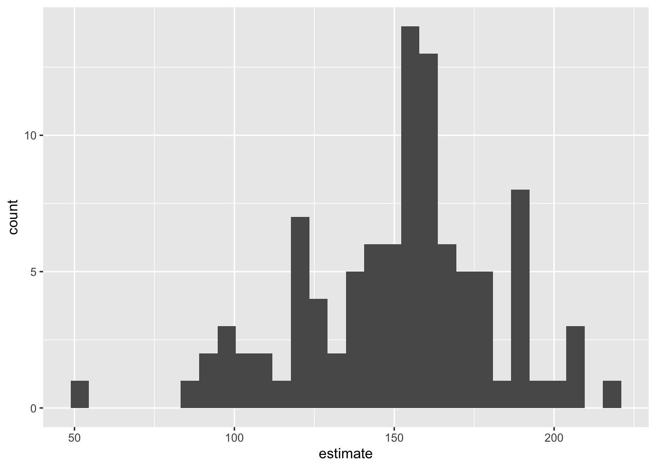
Computing the CI for the slope III
Percentile method: Compute the 95% CI as the middle 95% of the bootstrap distribution:
get_confidence_interval(
  boot_fits,
  point_estimate = observed_fit,
  level = 0.95,
  type = "percentile"
)
# A tibble: 2 × 3
term lower_ci upper_ci
<chr> <dbl> <dbl>
1 area 92.4 206.
2 intercept 7014. 285255.Precision vs. accuracy
If we want to be very certain that we capture the population parameter, should we use a wider or a narrower interval? What drawbacks are associated with using a wider interval?
. . .

Precision vs. accuracy
How can we get best of both worlds – high precision and high accuracy?
Changing confidence level
How would you modify the following code to calculate a 90% confidence interval? How would you modify it for a 99% confidence interval?
get_confidence_interval(
  boot_fits,
  point_estimate = observed_fit,
  level = 0.95,
  type = "percentile"
)
# A tibble: 2 × 3
term lower_ci upper_ci
<chr> <dbl> <dbl>
1 area 92.4 206.
2 intercept 7014. 285255.Changing confidence level
## confidence level: 90%
get_confidence_interval(
  boot_fits, point_estimate = observed_fit,
  level = 0.90, type = "percentile"
)
# A tibble: 2 × 3
term lower_ci upper_ci
<chr> <dbl> <dbl>
1 area 96.1 197.
2 intercept 20626. 268049.## confidence level: 99%
get_confidence_interval(
boot_fits, point_estimate = observed_fit,
level = 0.99, type = "percentile"
)# A tibble: 2 × 3
term lower_ci upper_ci
<chr> <dbl> <dbl>
1 area 69.7 214.
2 intercept -25879. 351614.Recap
Population: Complete set of observations of whatever we are studying, e.g., people, tweets, photographs, etc. (population size = \(N\))
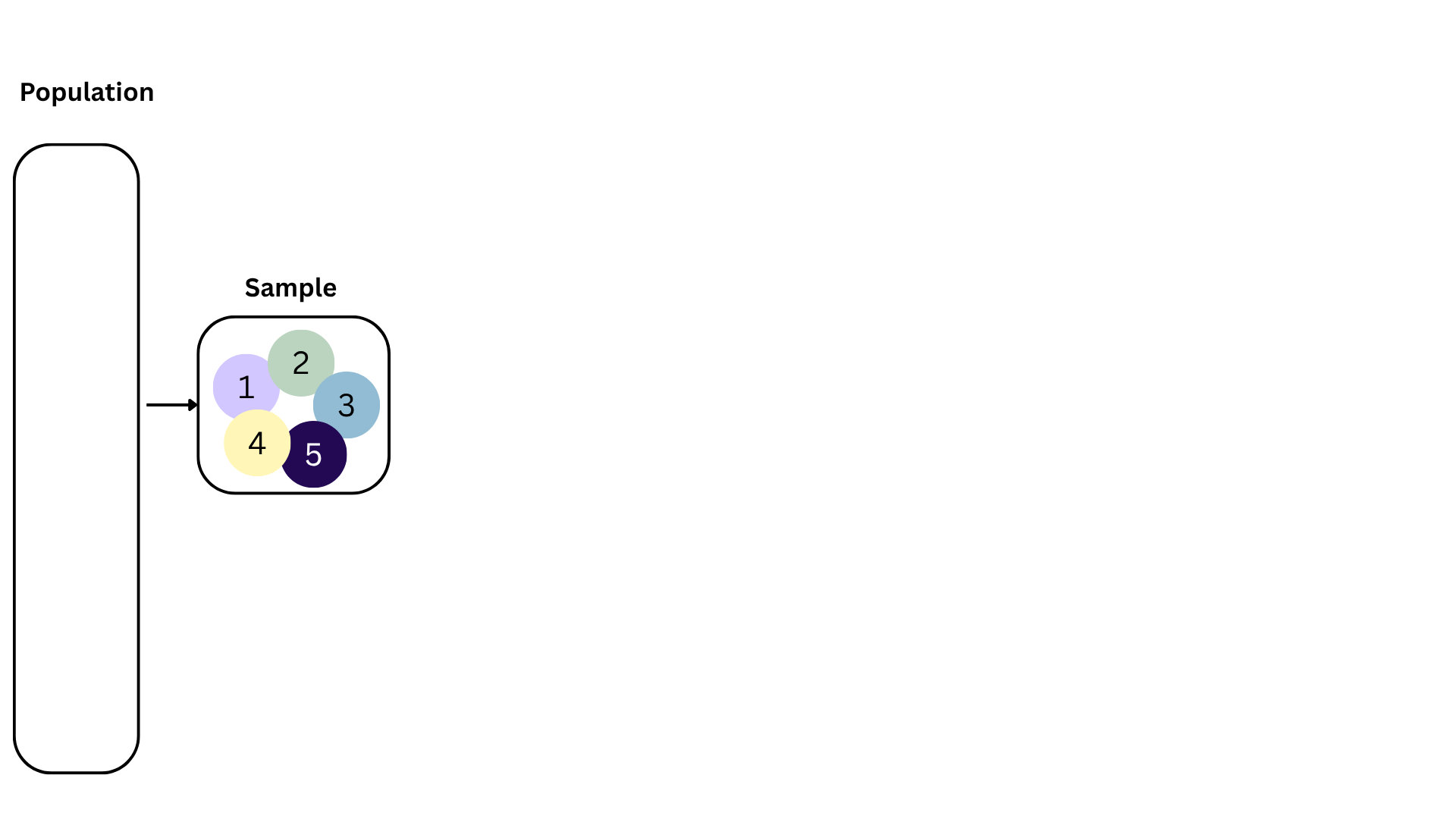
Sample: Subset of the population, ideally random and representative (sample size = \(n\))
Sample statistic \(\ne\) population parameter, but if the sample is good, it can be a good estimate
Statistical inference: Discipline that concerns itself with extracting meaning and information from data that has been generated by random process
We report the estimate with a confidence interval. The width of this interval depends on the variability of sample statistics from different samples from the population
Since we can’t continue sampling from the population, we bootstrap from the one sample we have to estimate sampling variability
  linear_reg() |>
    fit(wt ~ cyl + hp, data = mtcars)
parsnip model object
Call:
stats::lm(formula = wt ~ cyl + hp, data = data)
Coefficients:
(Intercept) cyl hp
0.5820880 0.4177733 0.0003422