Quantifying uncertainty with bootstrap intervals
Lecture 20
June 12, 2025
Confusion Matrix
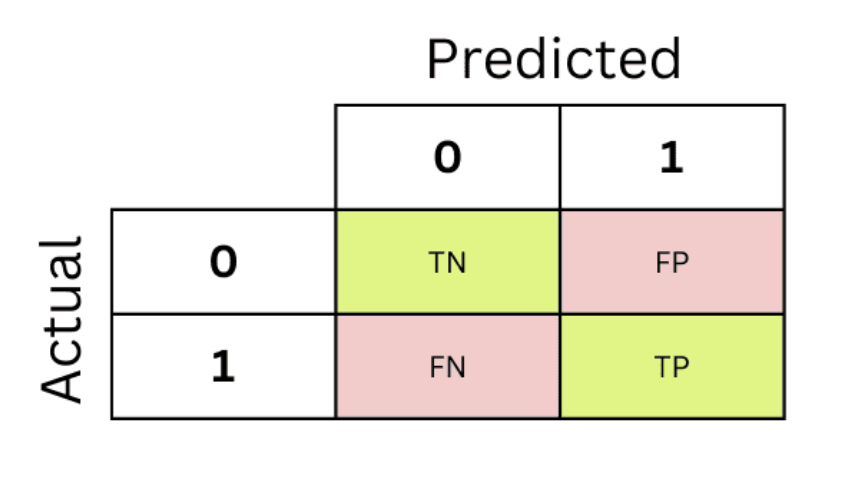
- False negative rate = \(\frac{FN}{FN + TP}\)
- False positive rate = \(\frac{FP}{FP + TN}\)
- Sensitivity = \(\frac{FN}{FN + TP}\) = 1 − False negative rate
- Specificity = \(\frac{TN}{FP + TN}\) = 1 - False positive rate
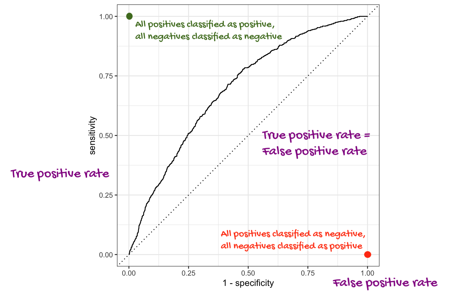
ROC Curve
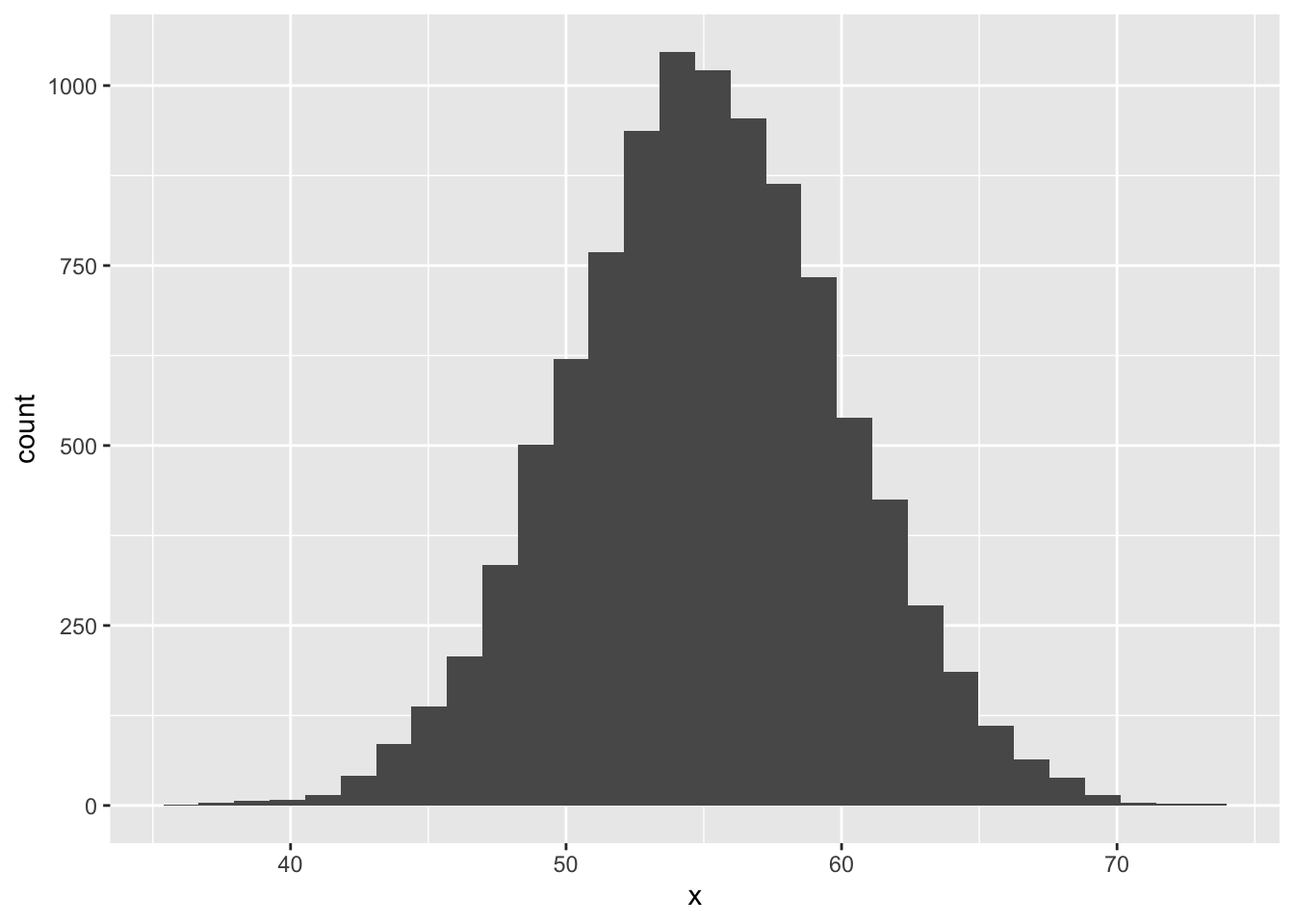
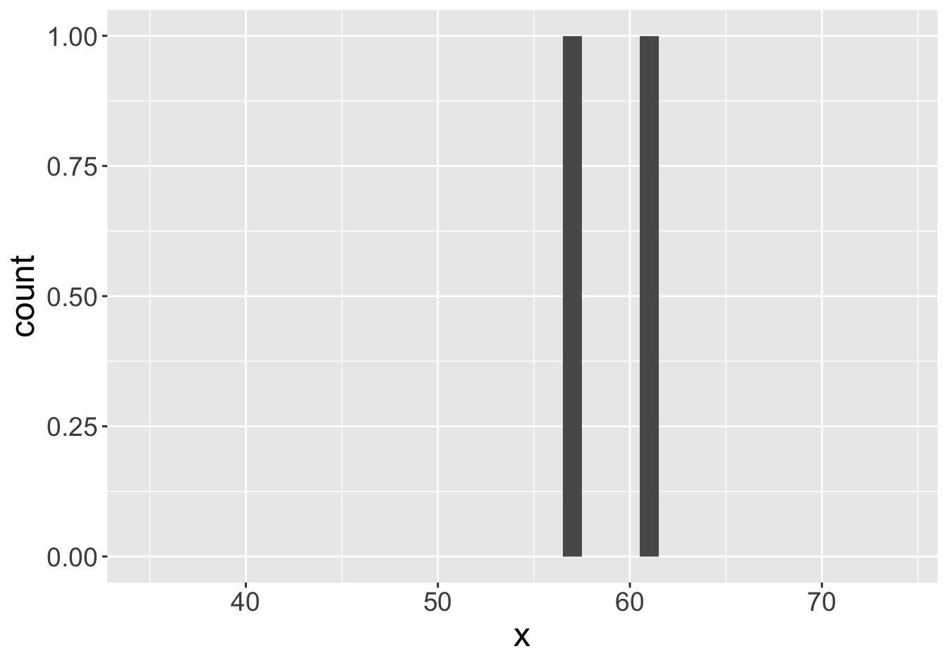
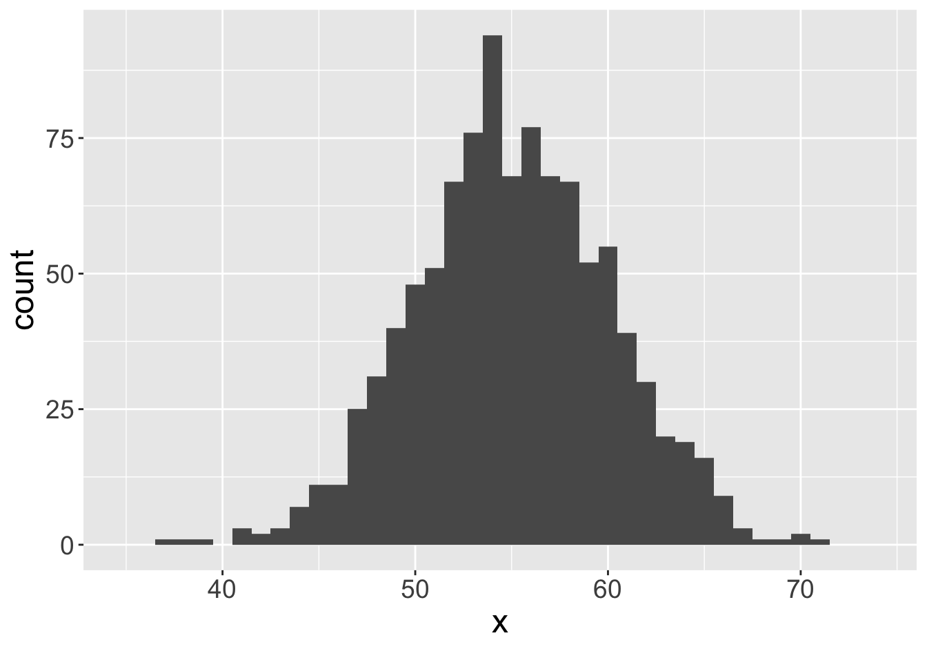
Example - Means (Sample Size 2)

Mean: 55.06
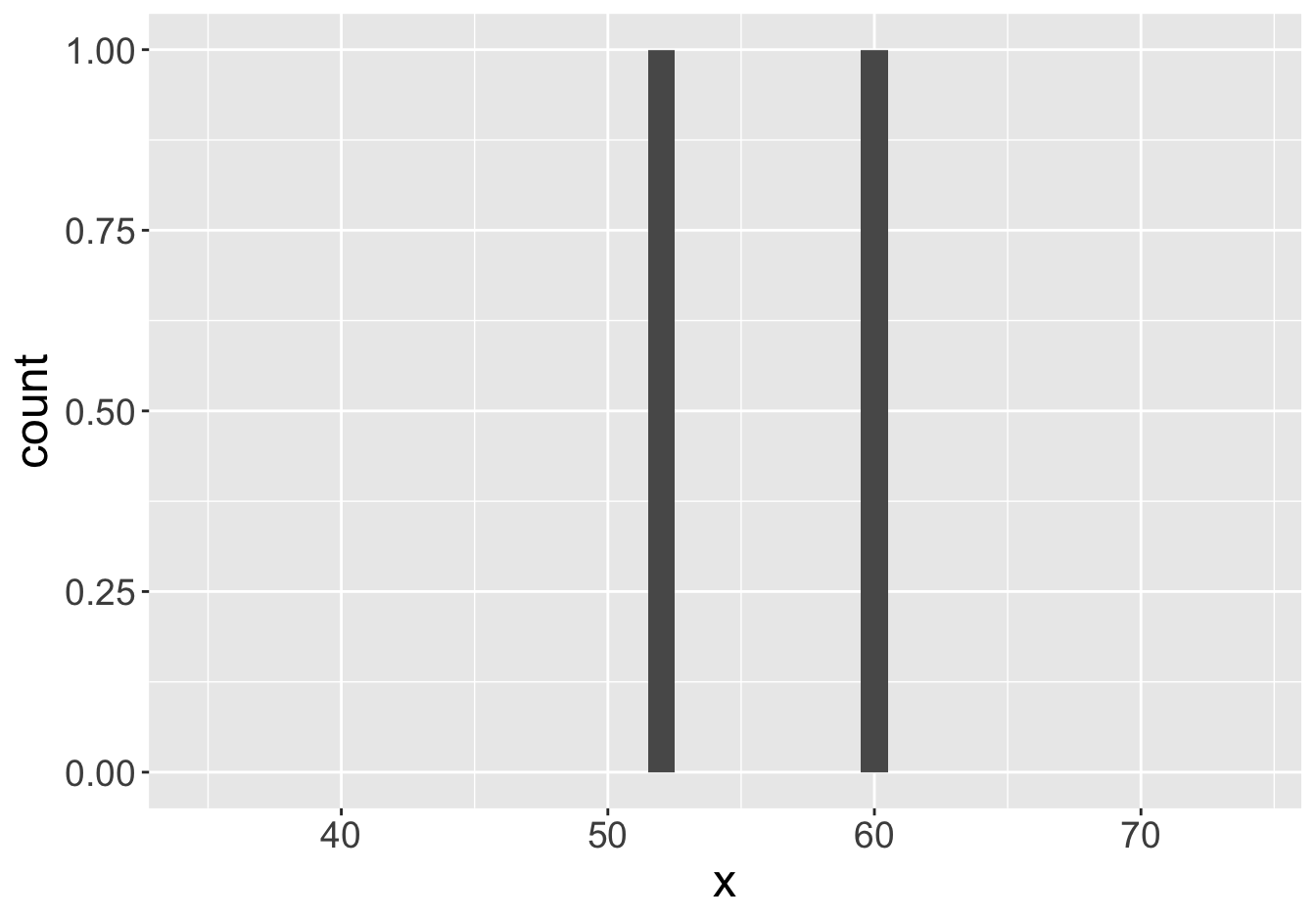
Mean: 55.9
Example - Means (Sample Size 2)

Mean: 55.06
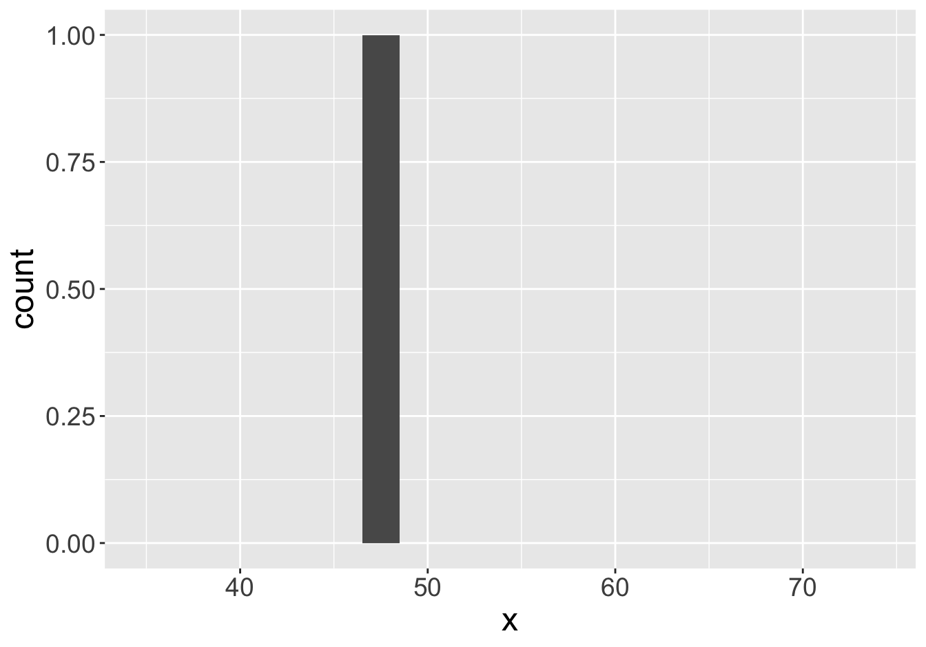
Mean: 47.8
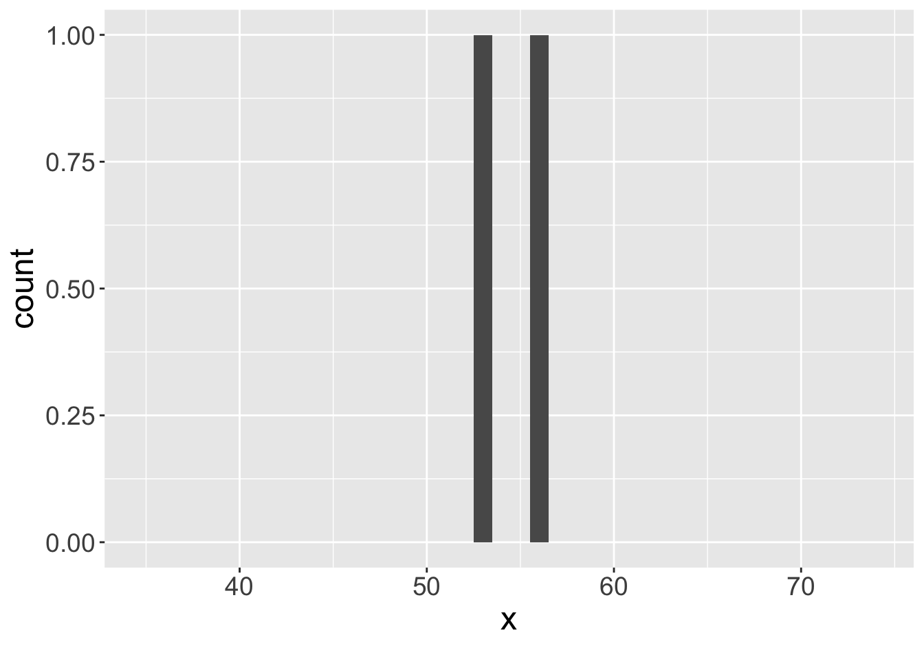
Example - Means (Sample Size 2)

Mean: 55.06
Mean: 56.08
Example - Means (Sample Size 2)

Mean: 55.06
Mean: 54.38
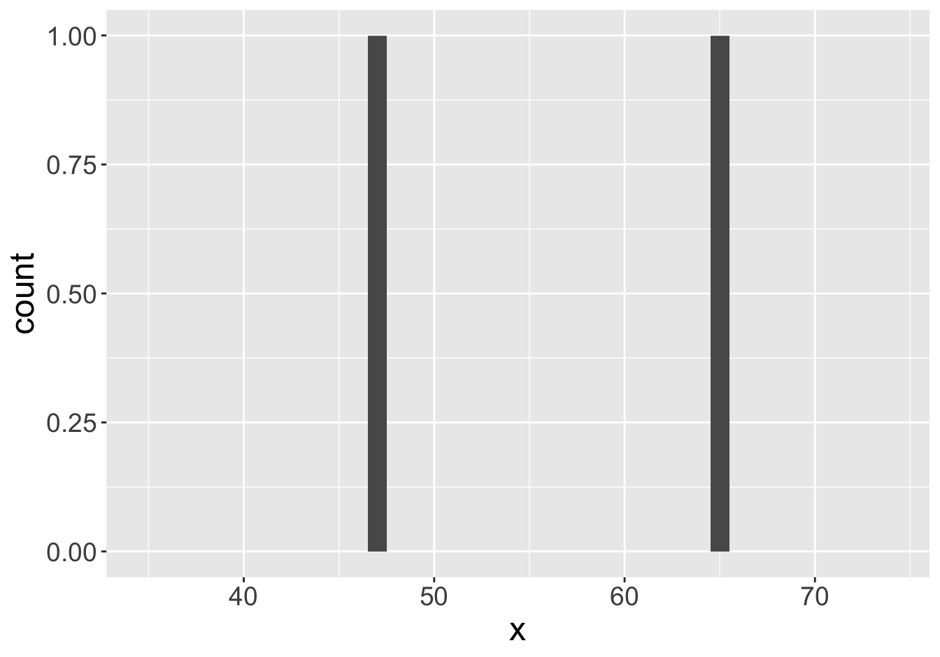
Example - Means (Sample Size 2)

Mean: 55.06
Mean: 59.24
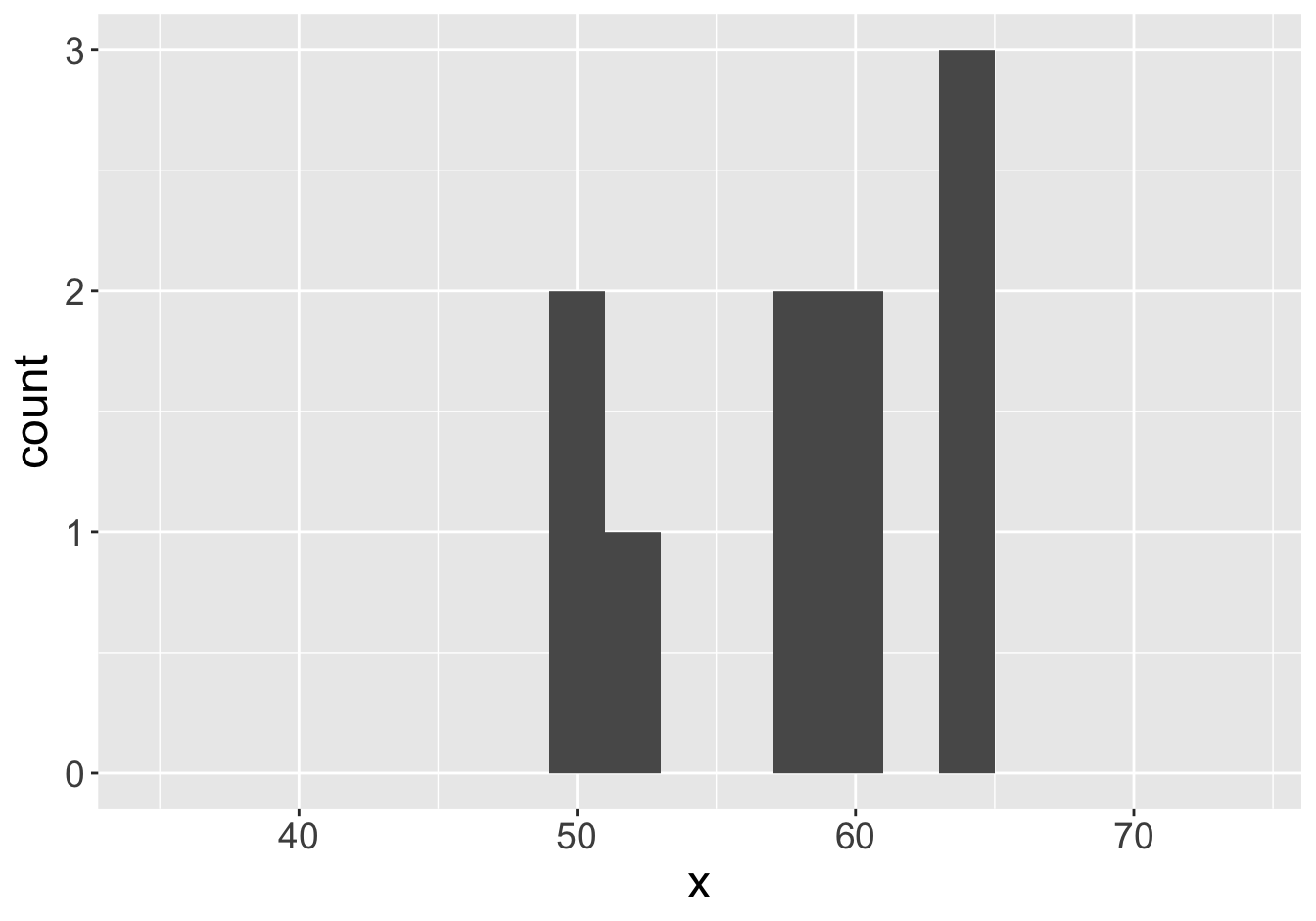
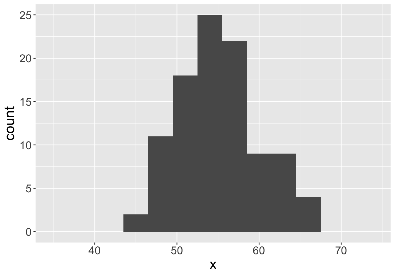
Example - Means (Sample Size 10)

Mean: 55.06
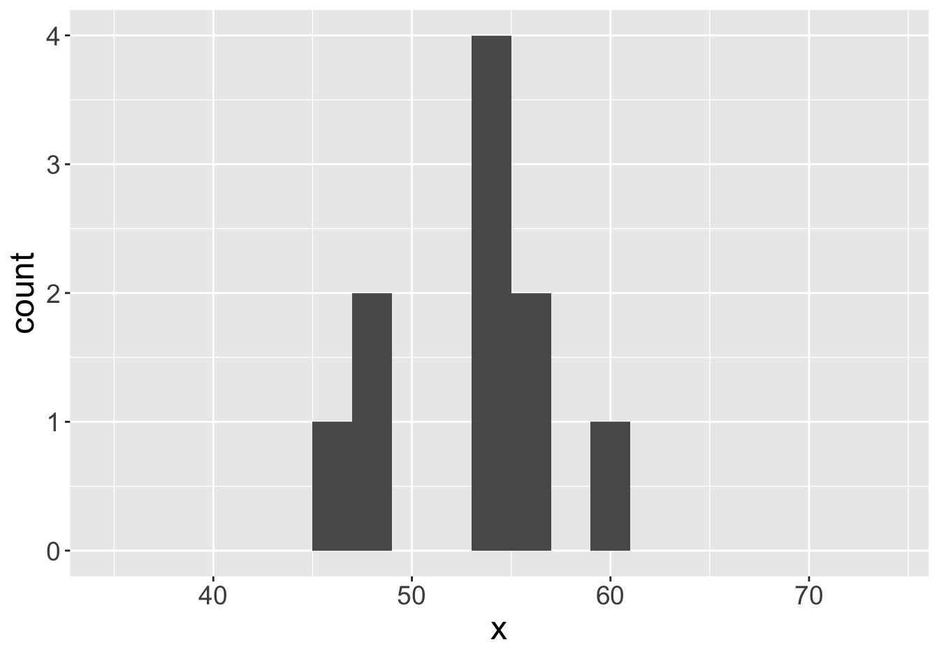
Mean: 53.29
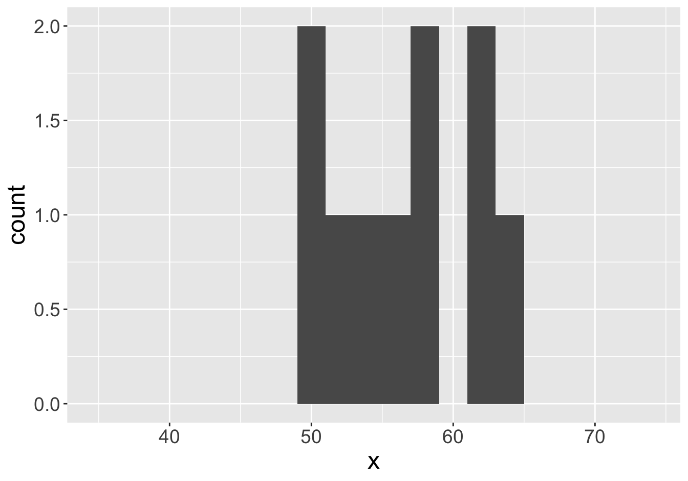
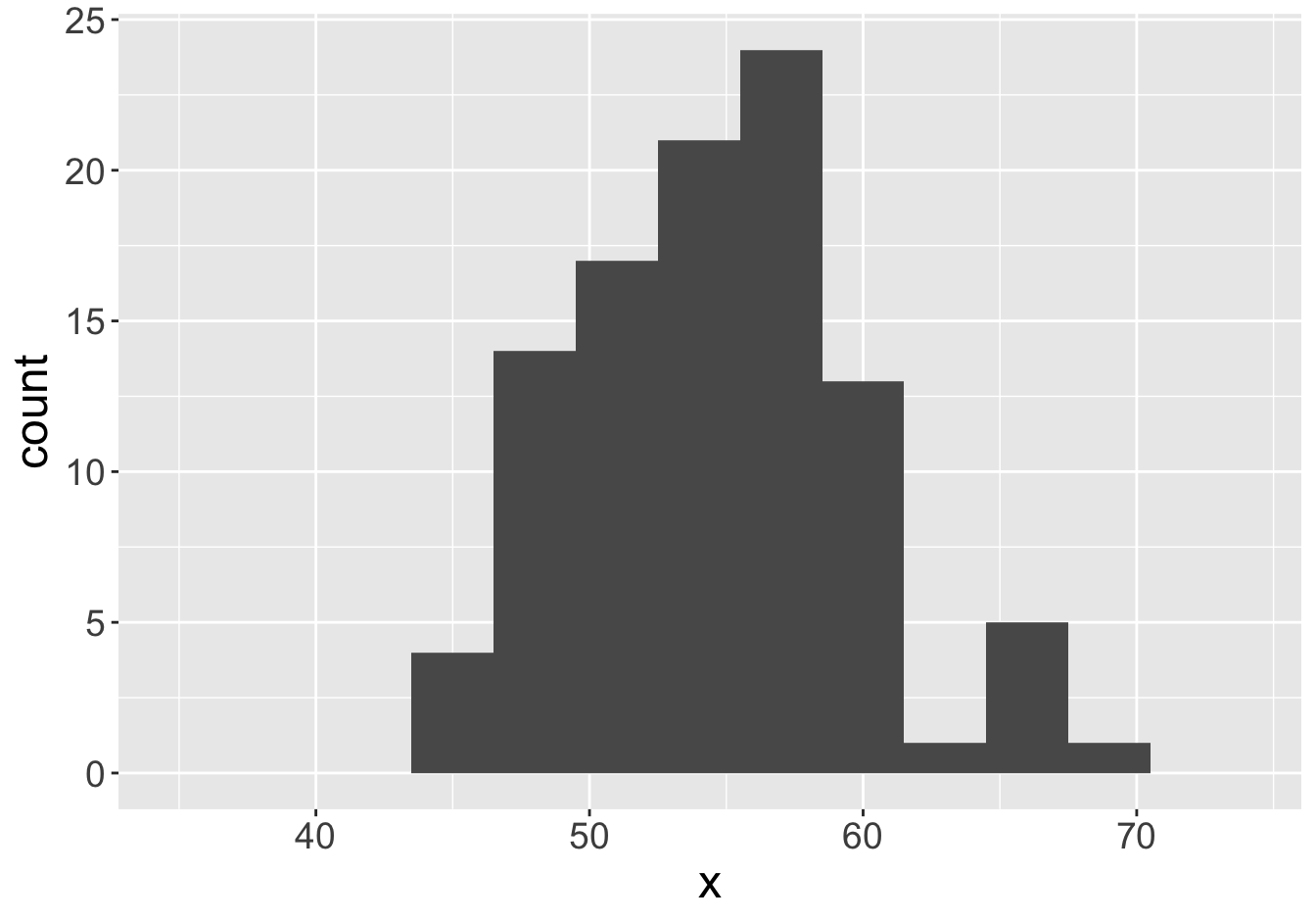
Example - Means (Sample Size 10)

Mean: 55.06
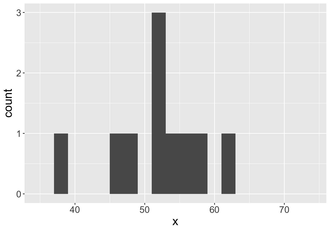
Mean: 51.59
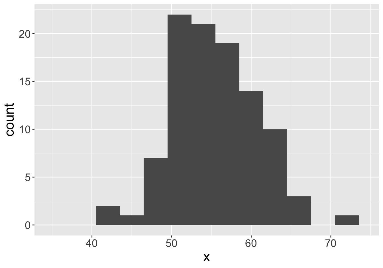
Example - Means (Sample Size 10)

Mean: 55.06
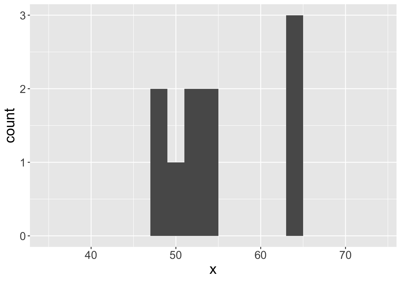
Mean: 55.24
Example - Means (Sample Size 10)

Mean: 55.06
Mean: 57.99
Example - Means (Sample Size 10)

Mean: 55.06
Mean: 56.54
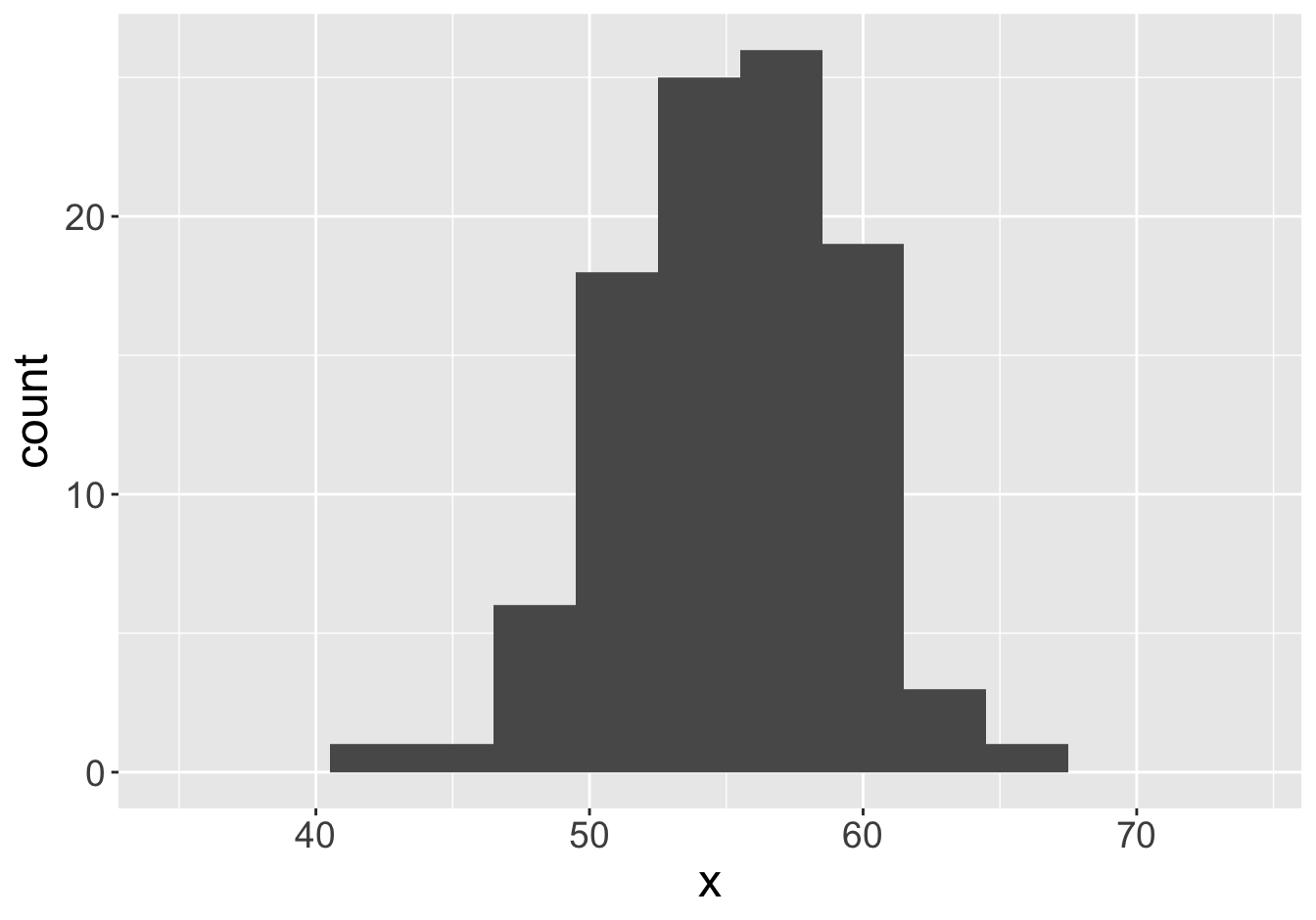
Example - Means (Sample Size 100)

Mean: 55.06
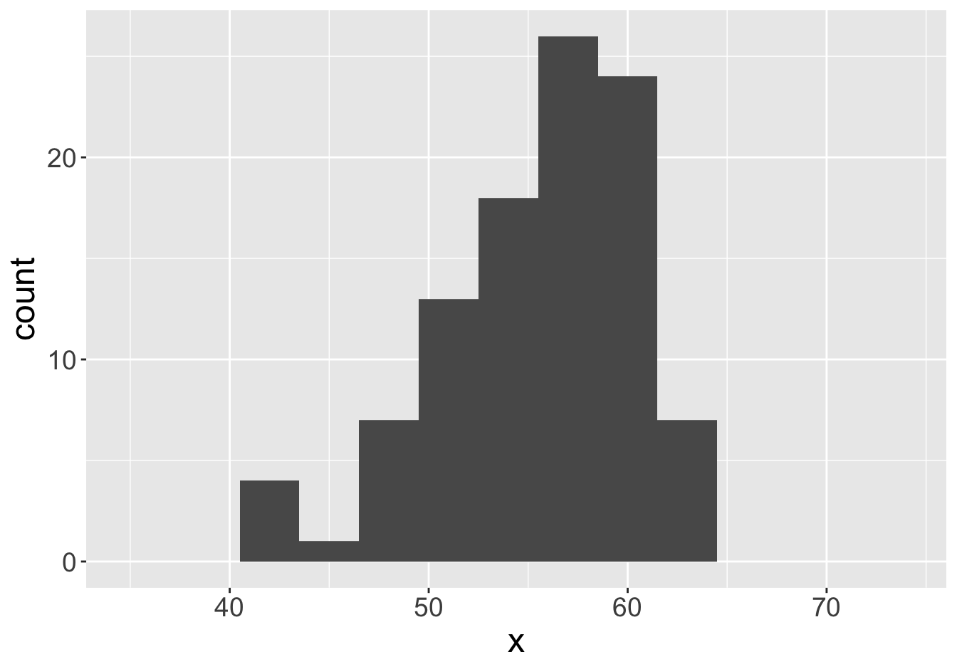
Mean: 55.55
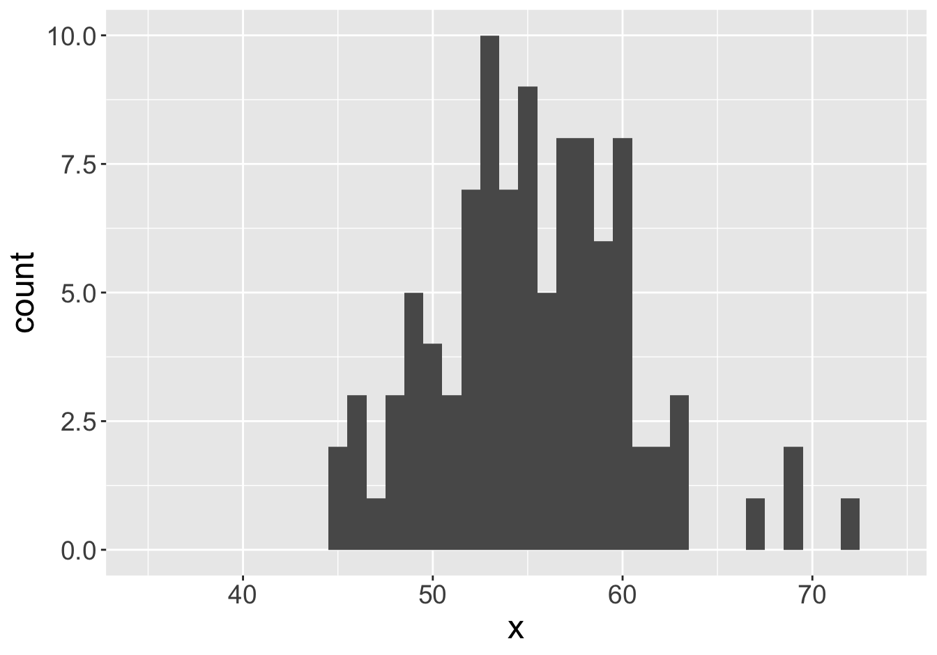
Example - Means (Sample Size 100)

Mean: 55.06
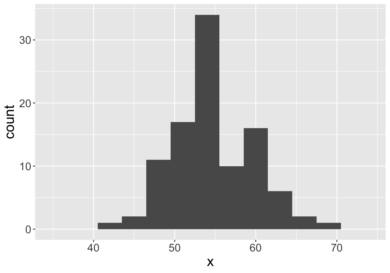
Mean: 54.84
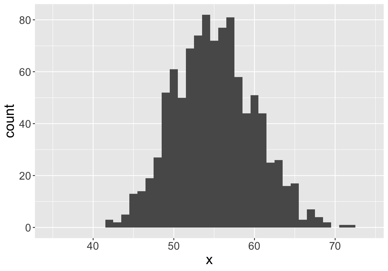
Example - Means (Sample Size 100)

Mean: 55.06
Mean: 54.98
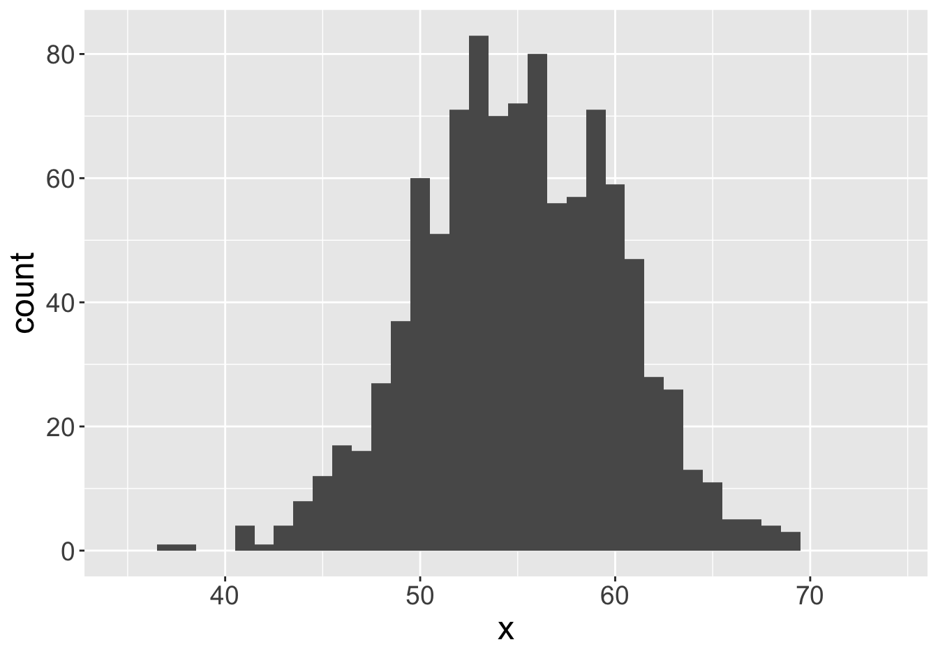
Example - Means (Sample Size 100)

Mean: 55.06
Mean: 54.58
Example - Means (Sample Size 100)
Mean: 55.06
Mean: 55.57
Example - Means (Sample Size 100)

Mean: 55.06
Mean: 55.12
Example - Means (Sample Size 100)

Mean: 55.06
Mean: 55.29
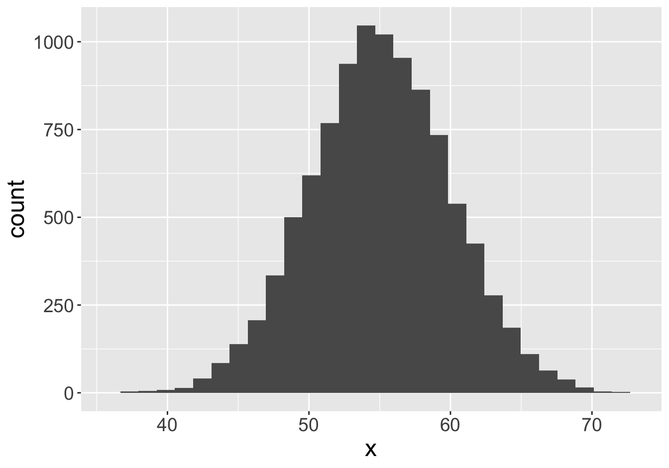
Example - Means (Sample Size 1000)

Mean: 55.06
Mean: 55.07
Example - Means (Sample Size 1000)

Mean: 55.06
Mean: 55.06
Example - Means (Sample Size 1000)

Mean: 55.06
Mean: 55.05
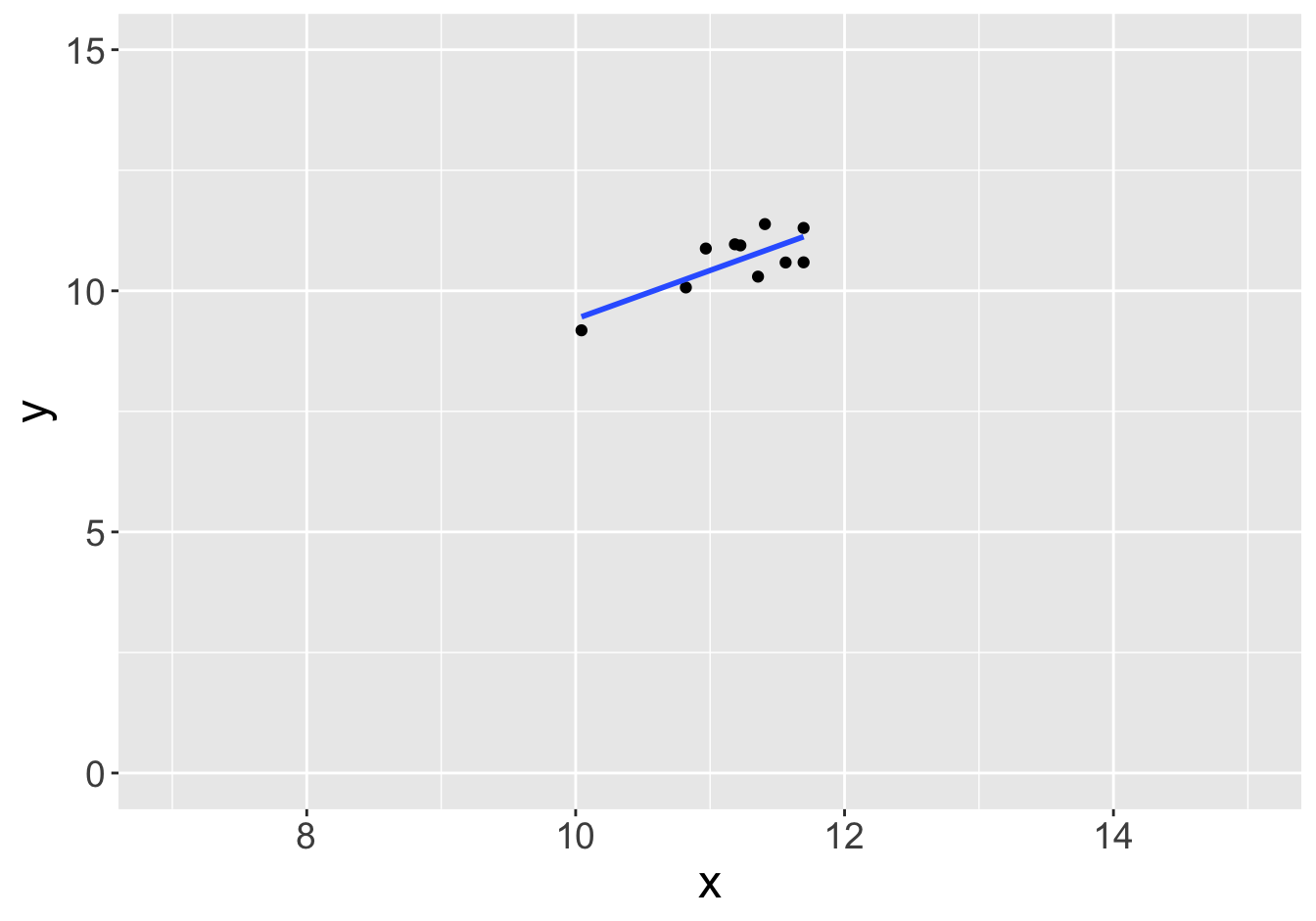
Example - Slopes
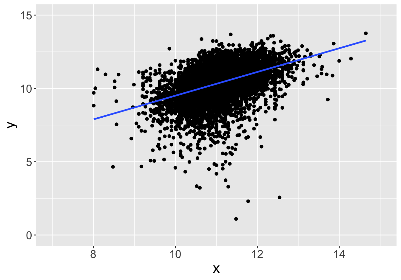
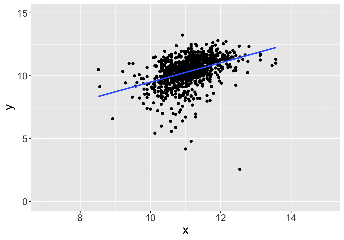
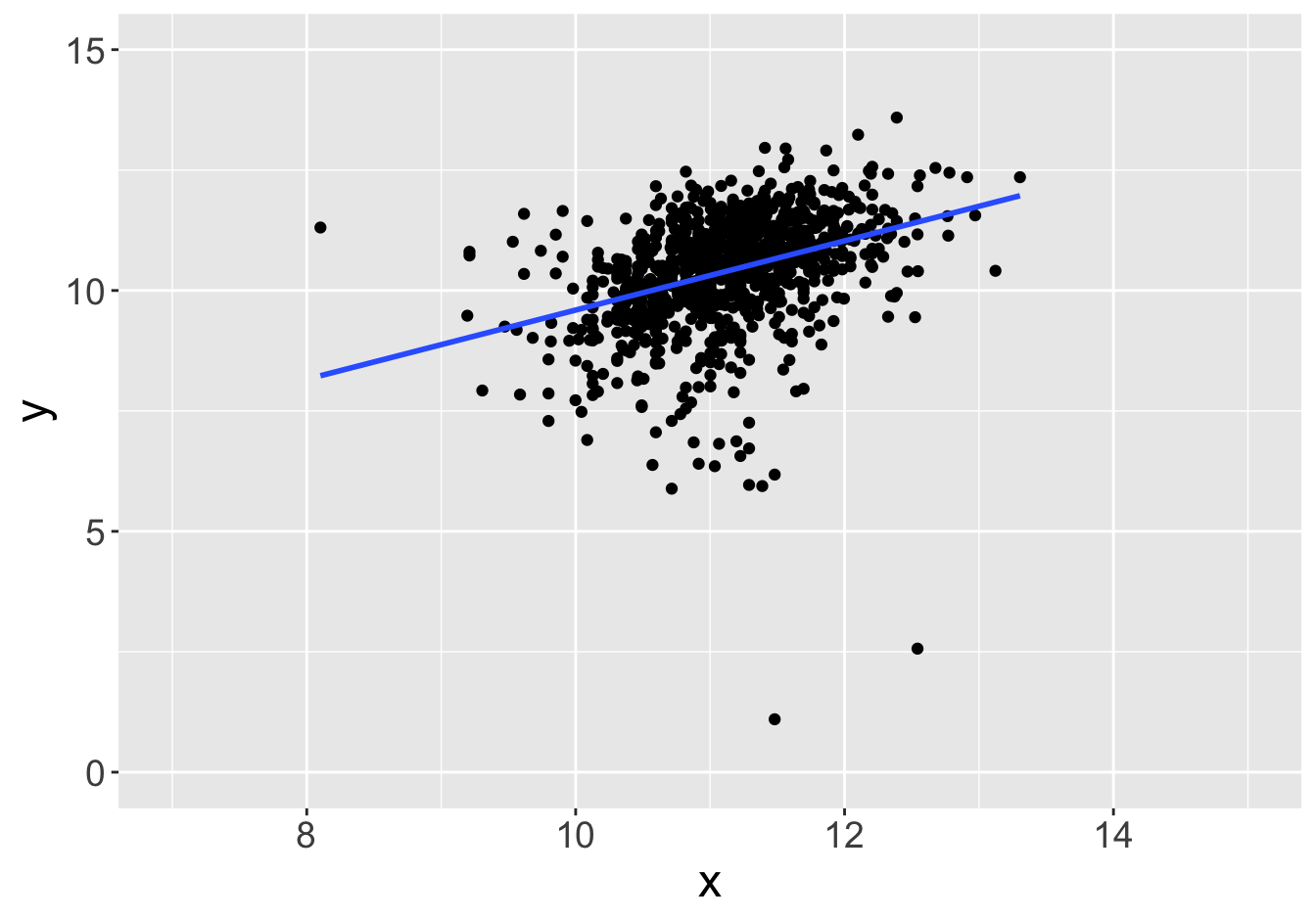
Suppose this scatter plot represents some values \(x, y\) in a population of 10,000:
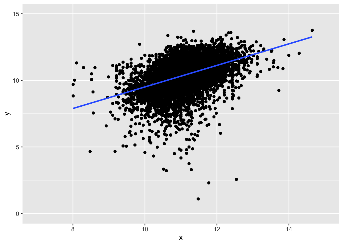
Slope: 0.81
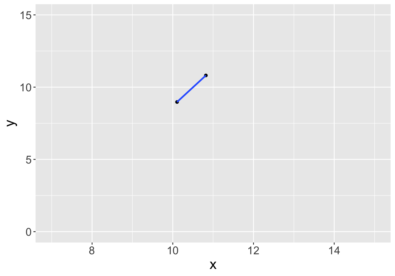
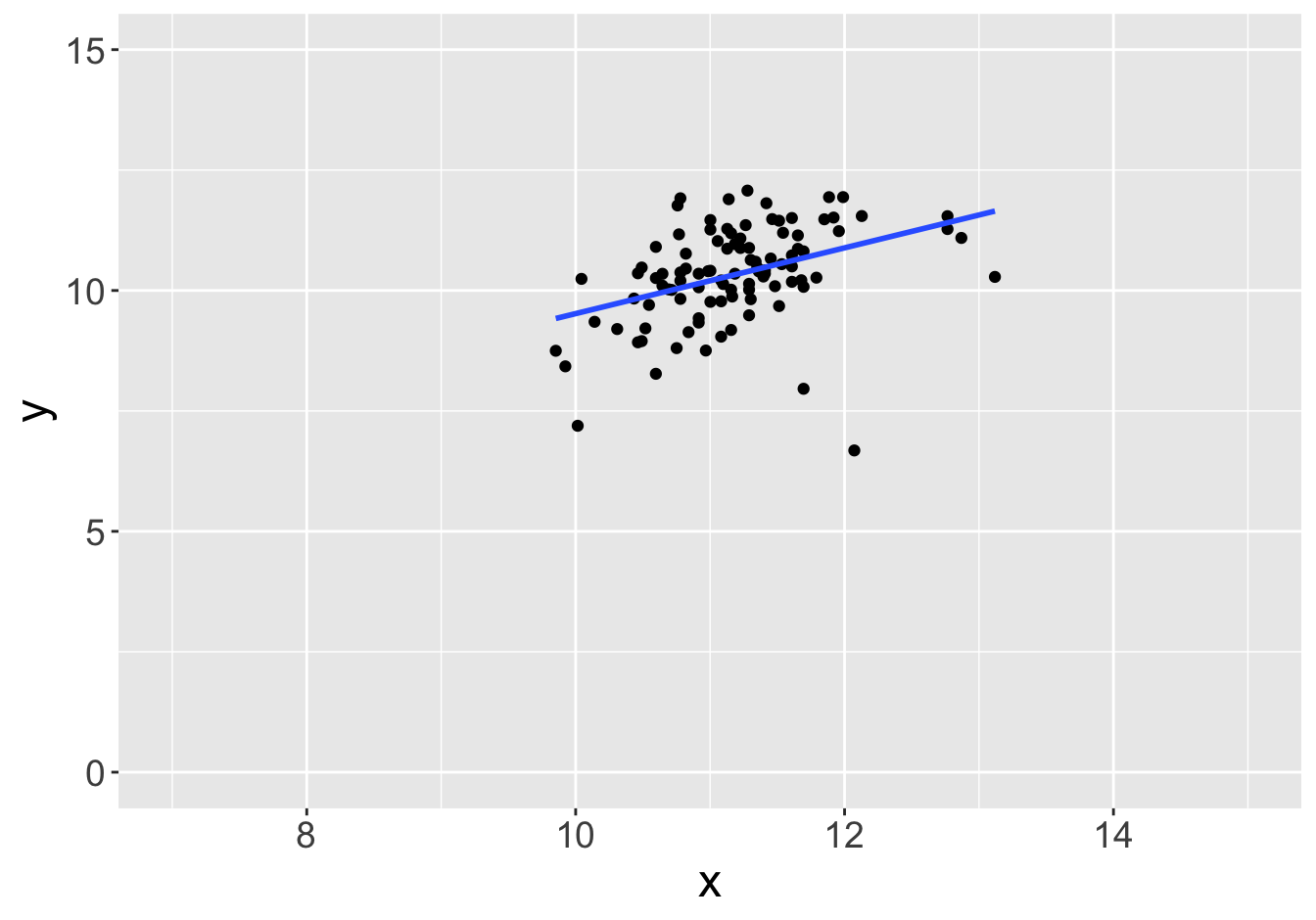
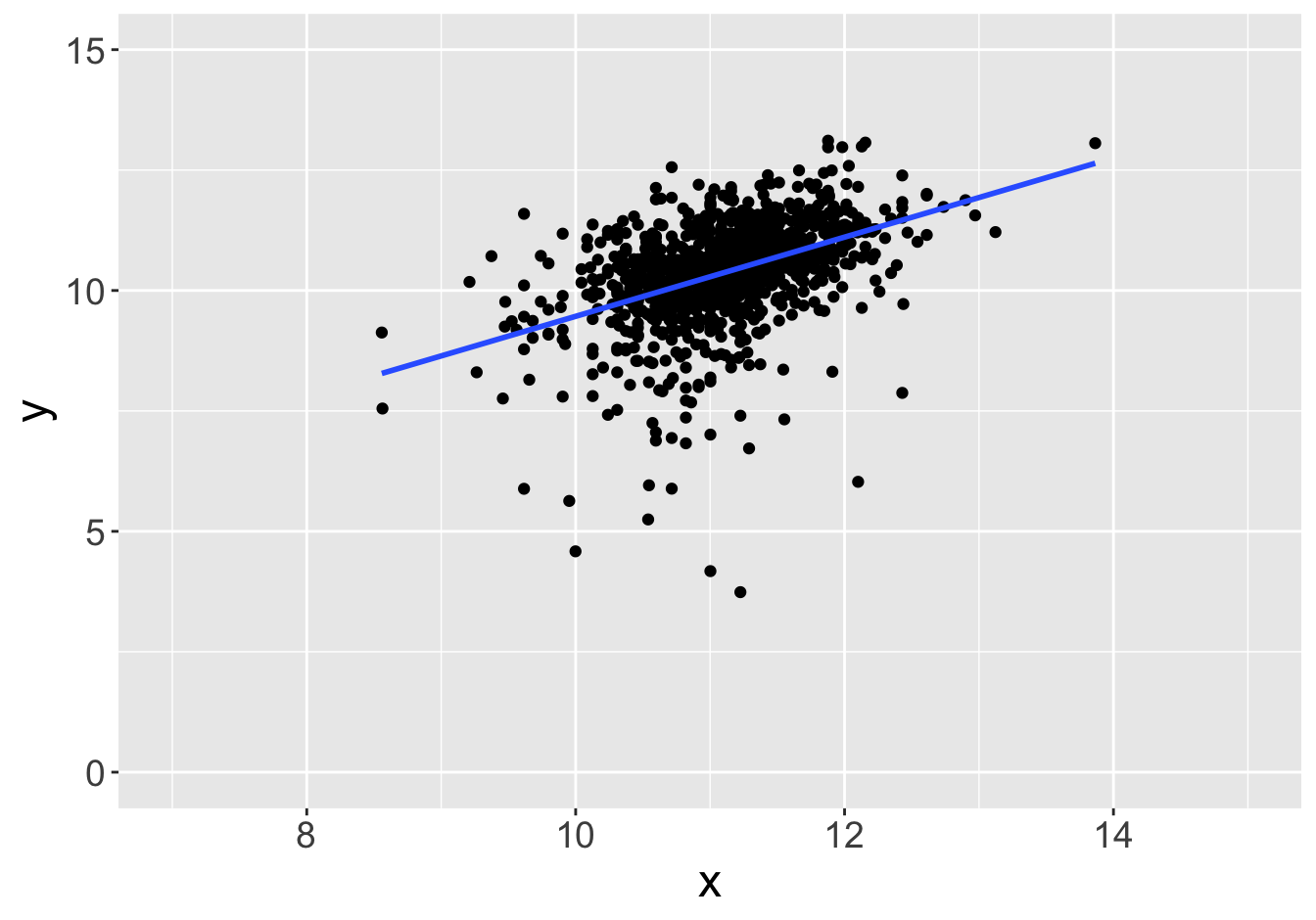
Example - Slopes (Sample Size 2)

Slope: 0.81
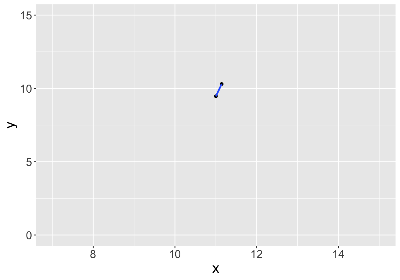
Slope: 5.97
Example - Slopes (Sample Size 2)

Slope: 0.81
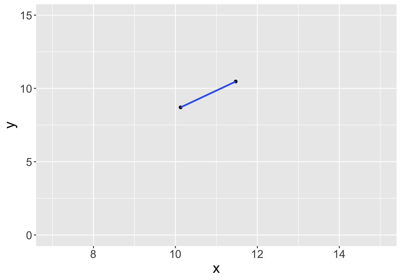
Slope: 1.31
Example - Slopes (Sample Size 2)

Slope: 0.81
Slope: 2.57
Example - Slopes (Sample Size 2)

Slope: 0.81
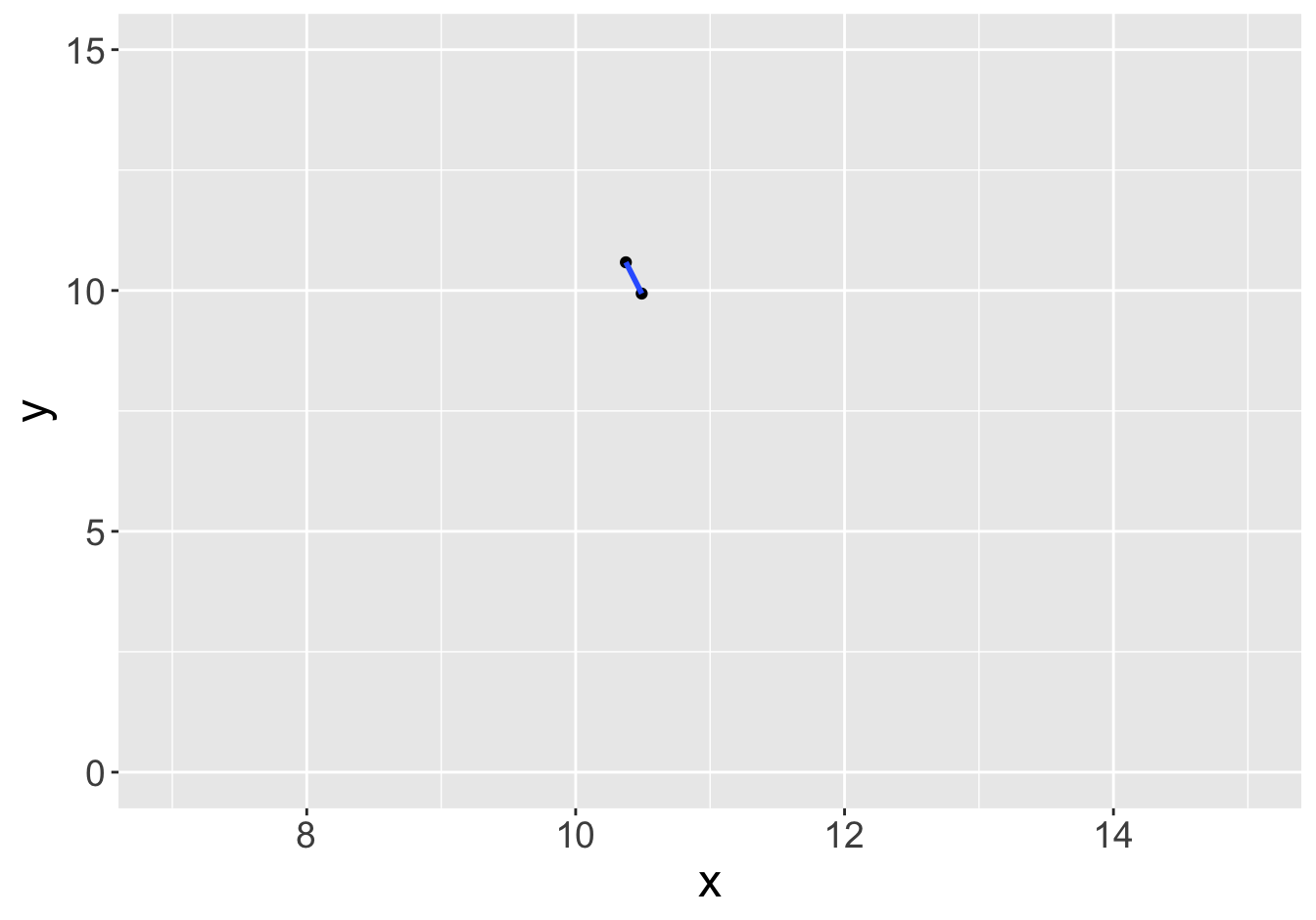
Slope: -5.51
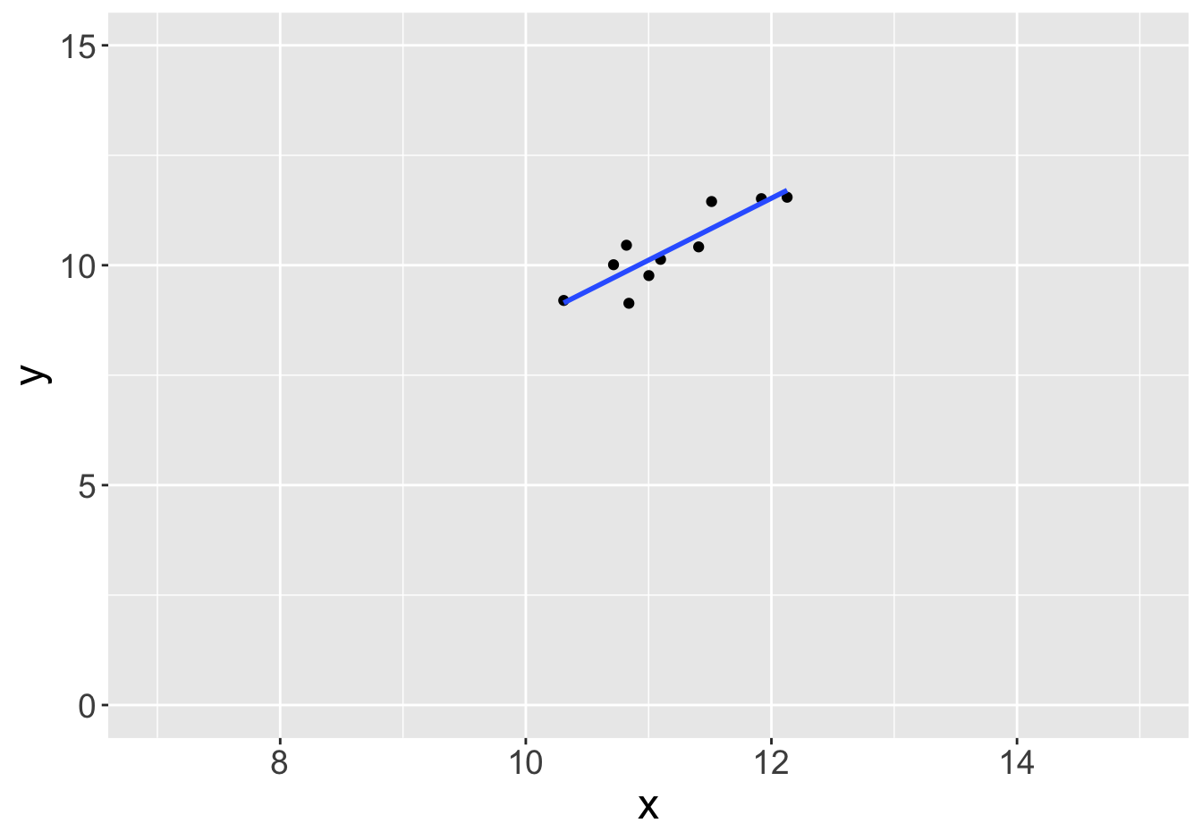
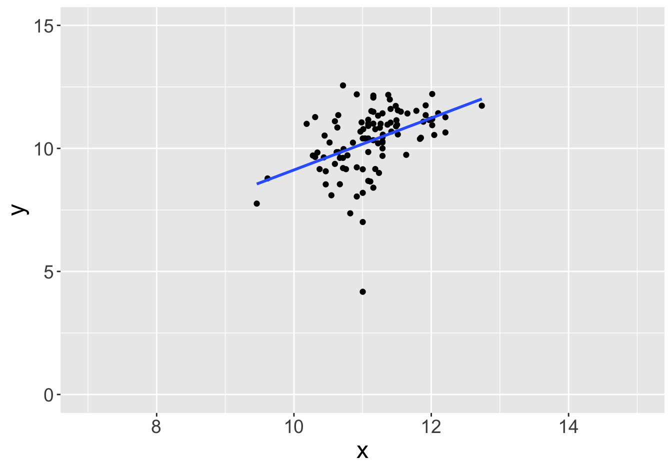
Example - Slopes (Sample Size 10)

Slope: 0.81
Slope: 1.08
Example - Slopes (Sample Size 10)
Slope: 0.81
Slope: 1.01
Example - Slopes (Sample Size 10)

Slope: 0.81
Slope: 1.41
Example - Slopes (Sample Size 10)

Slope: 0.81
Slope: 0.45
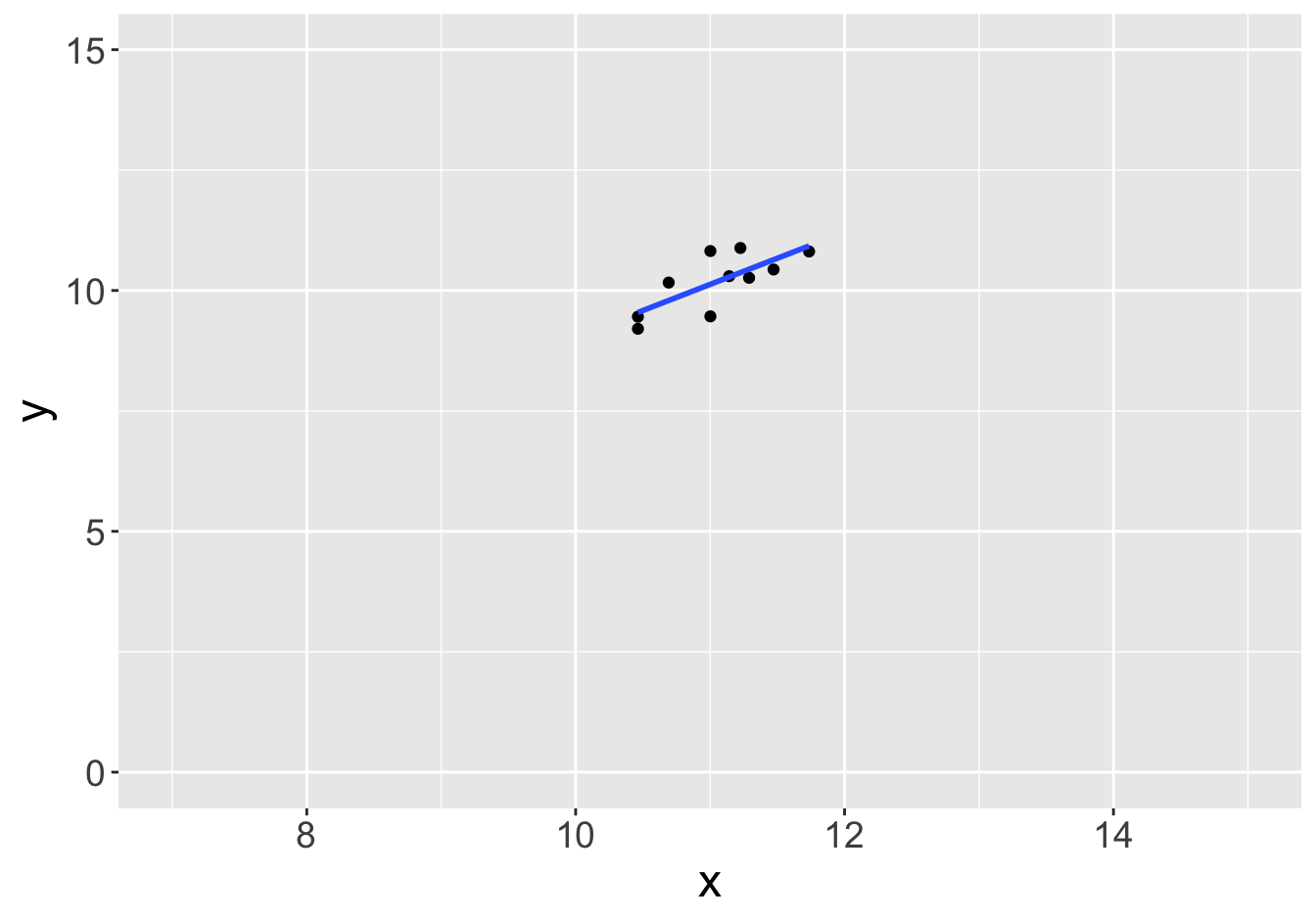
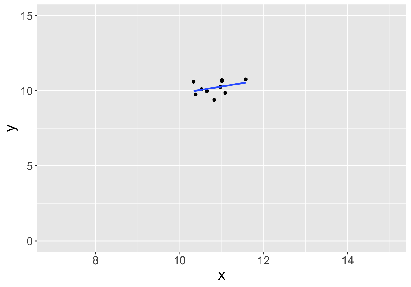
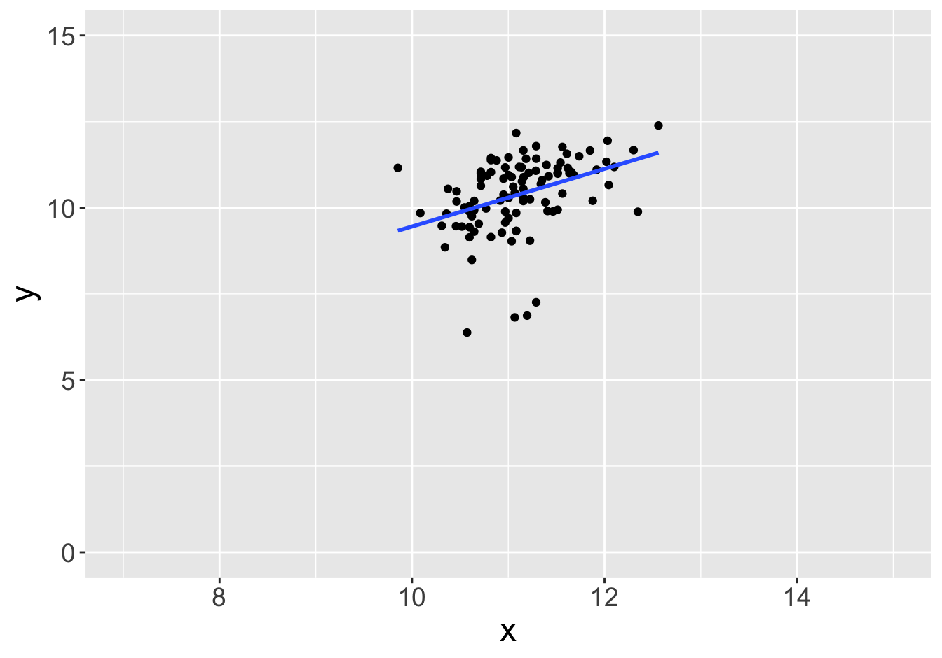
Example - Slopes (Sample Size 100)

Slope: 0.81
Slope: 1.06
Example - Slopes (Sample Size 100)

Slope: 0.81
Slope: 0.68
Example - Slopes (Sample Size 100)

Slope: 0.81
Slope: 1.05
Example - Slopes (Sample Size 100)

Slope: 0.81
Slope: 0.84
Example - Slopes (Sample Size 100)

Slope: 0.81

Slope: 0.64
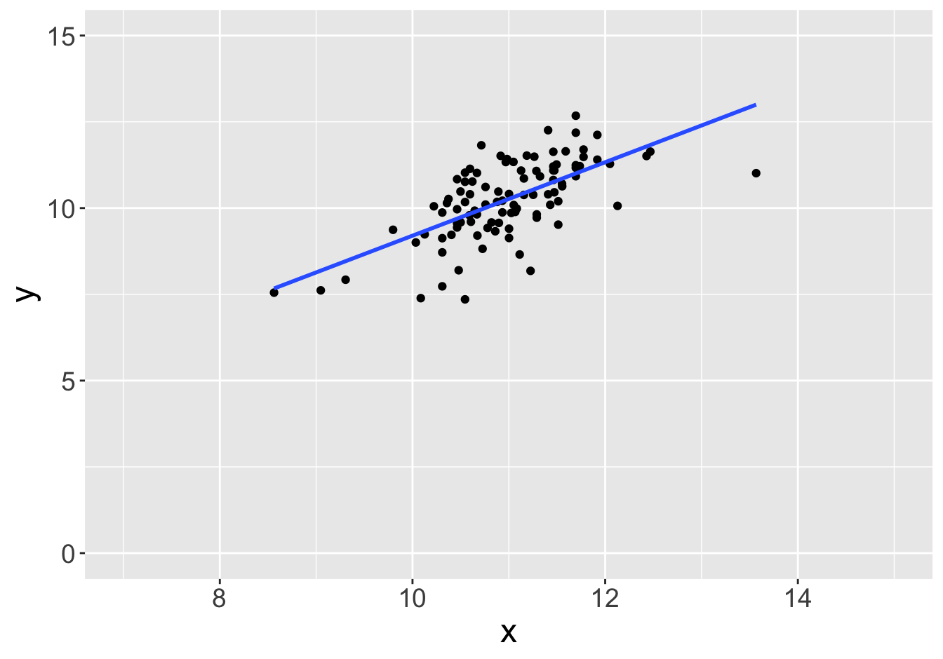
Example - Slopes (Sample Size 1000)

Slope: 0.81
Slope: 0.77
Example - Slopes (Sample Size 1000)

Slope: 0.81
Slope: 0.72
Example - Slopes (Sample Size 1000)

Slope: 0.81
Slope: 0.82
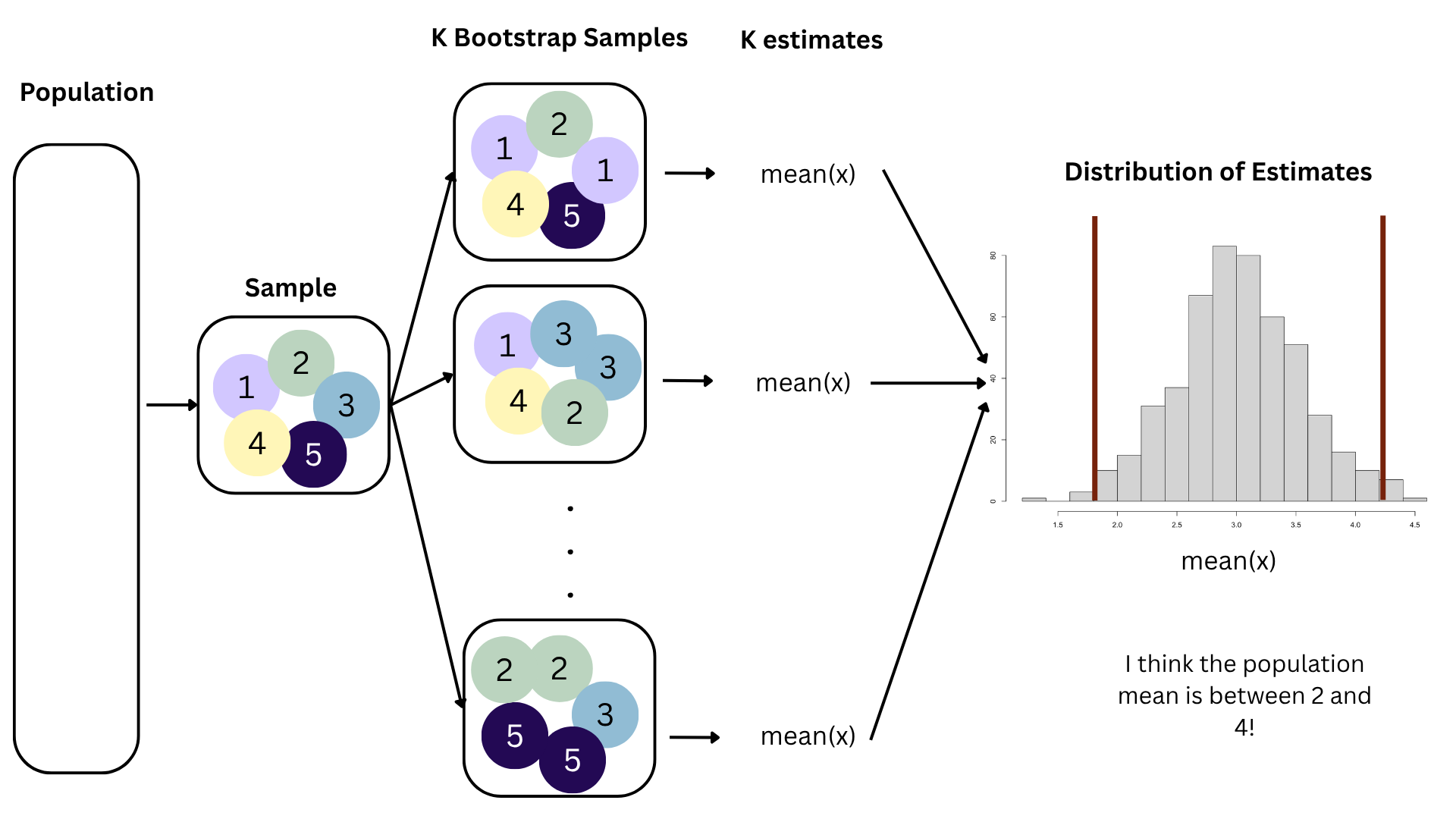
Bootstrapping
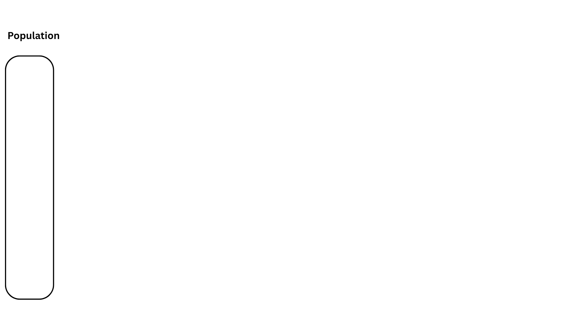
Bootstrapping
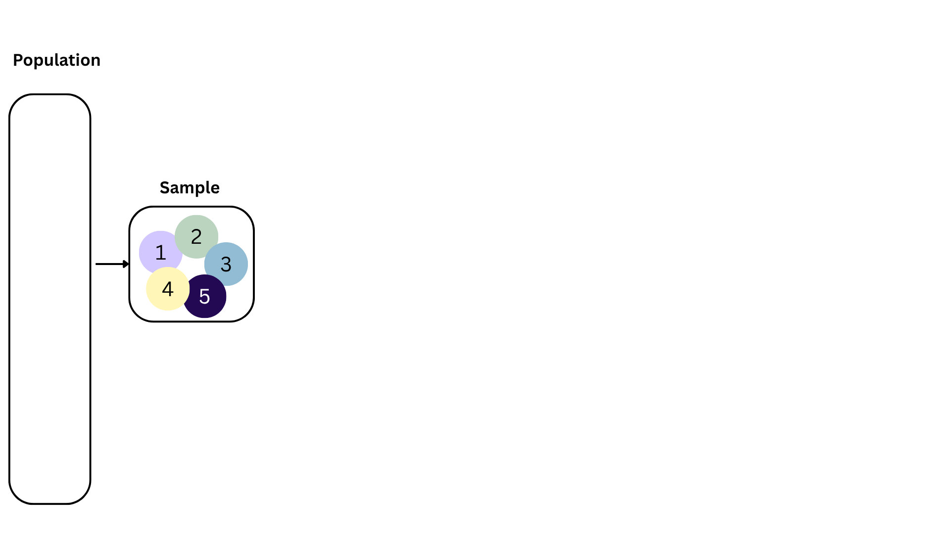
Bootstrapping
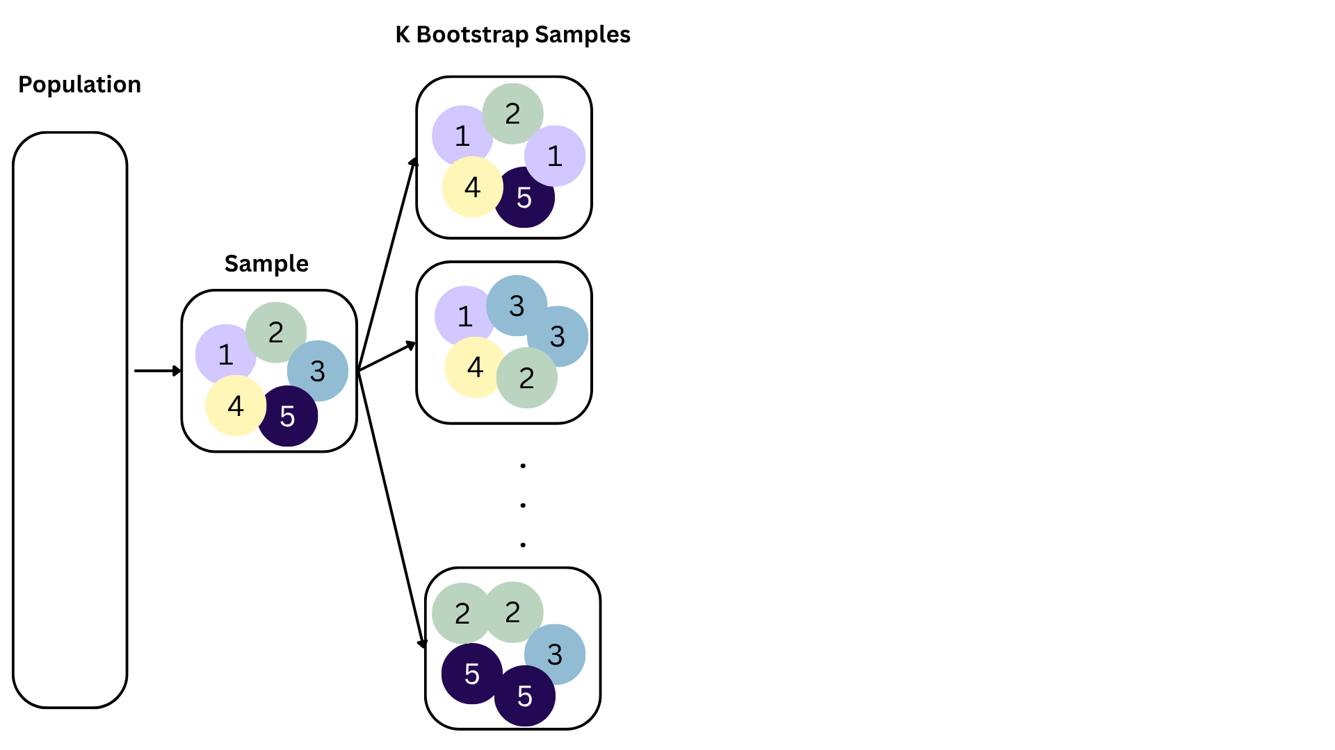
Bootstrapping
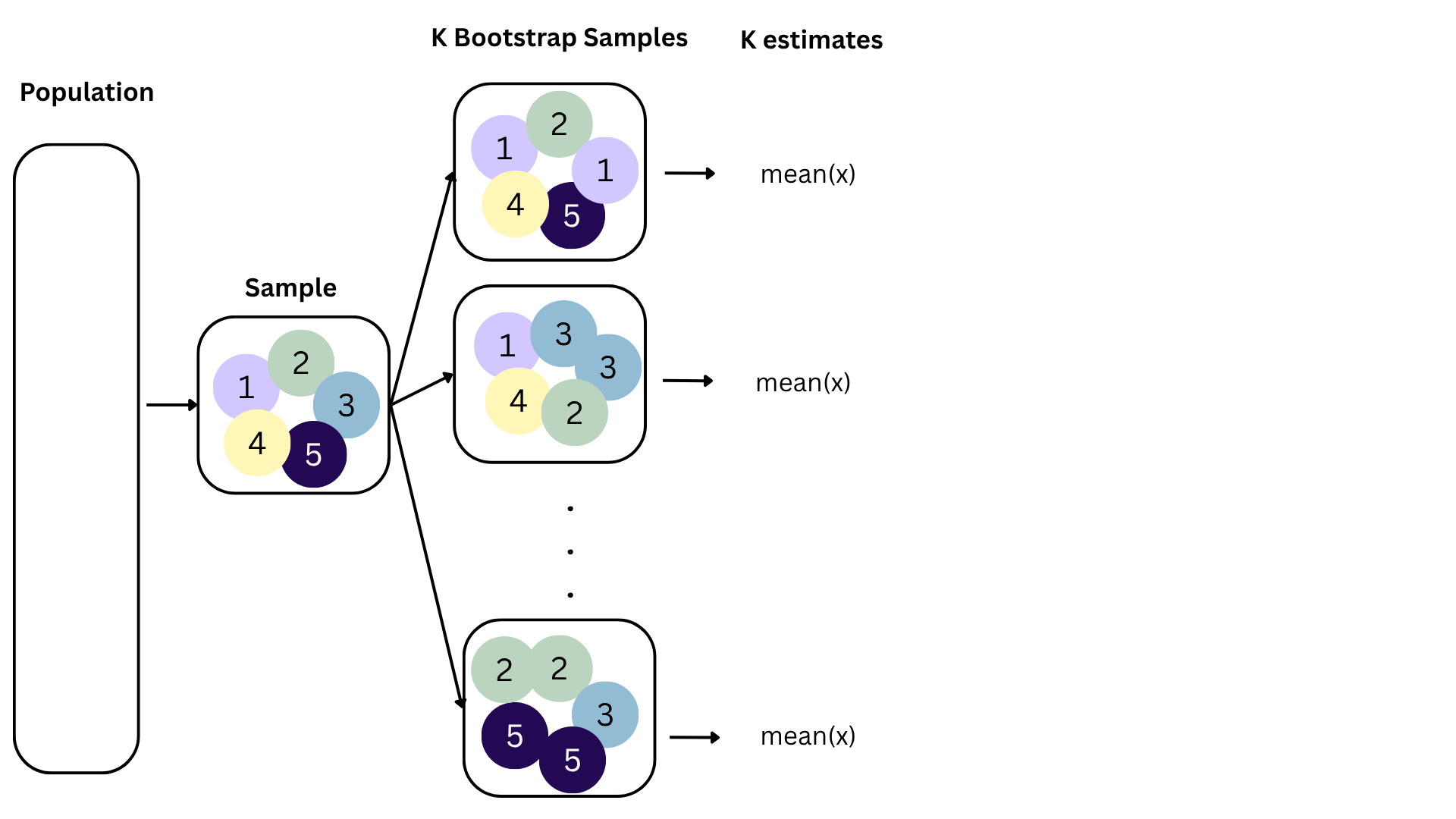
Bootstrapping
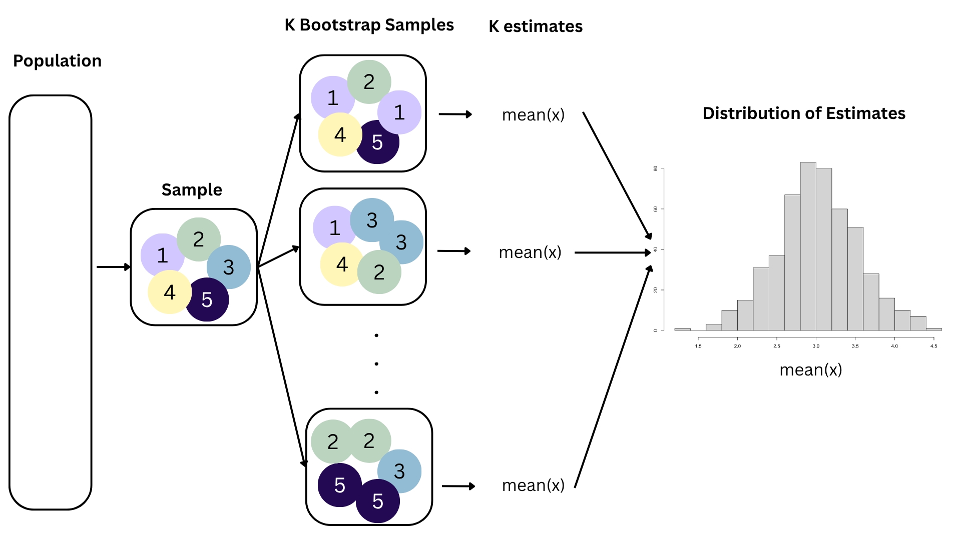
Bootstrapping
Bootstrapping
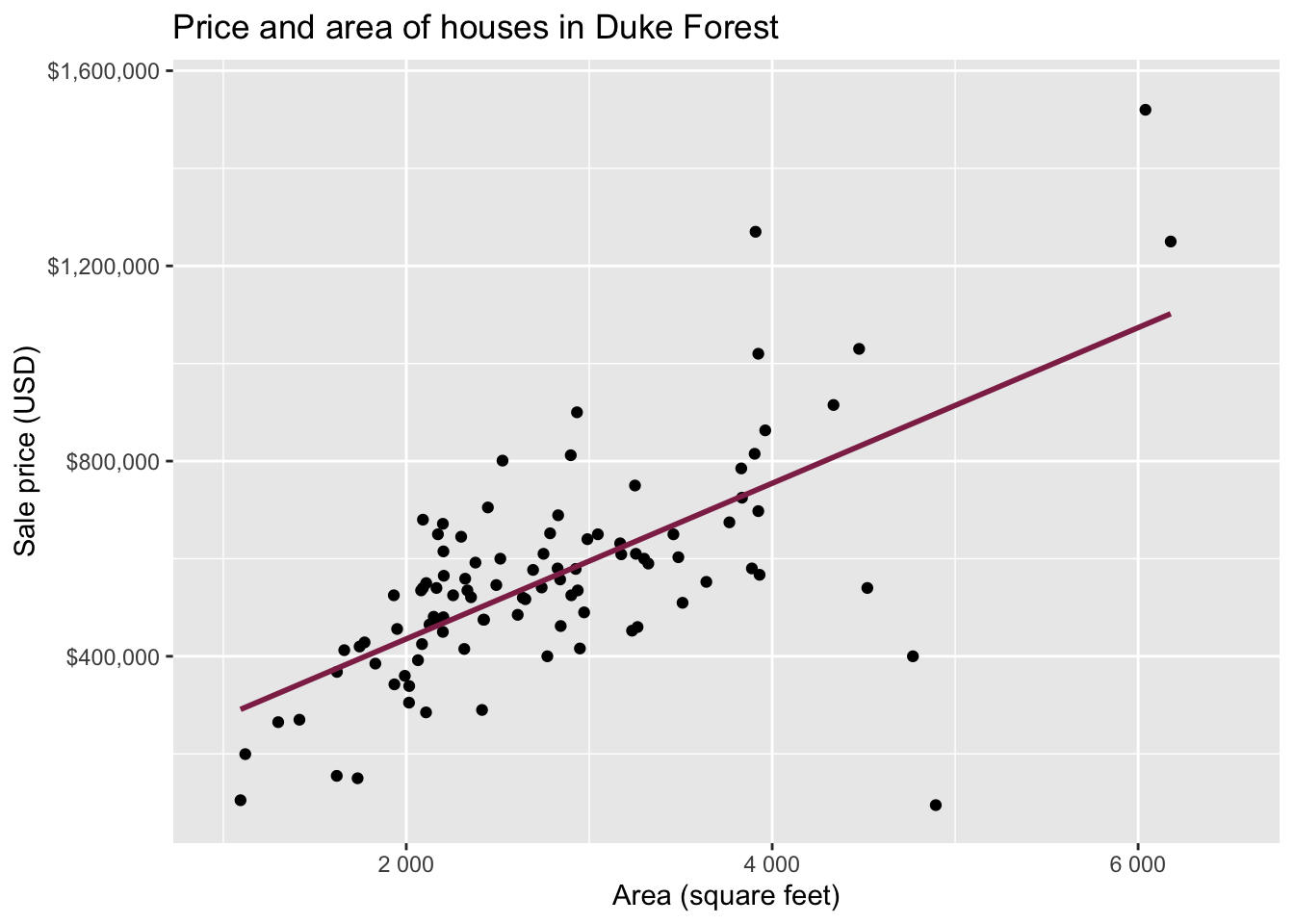
Data: Houses in Duke Forest
- Data on houses that were sold in the Duke Forest neighborhood of Durham, NC around November 2020
- Pulled from Zillow
- Source:
openintro::duke_forest
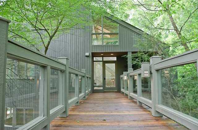
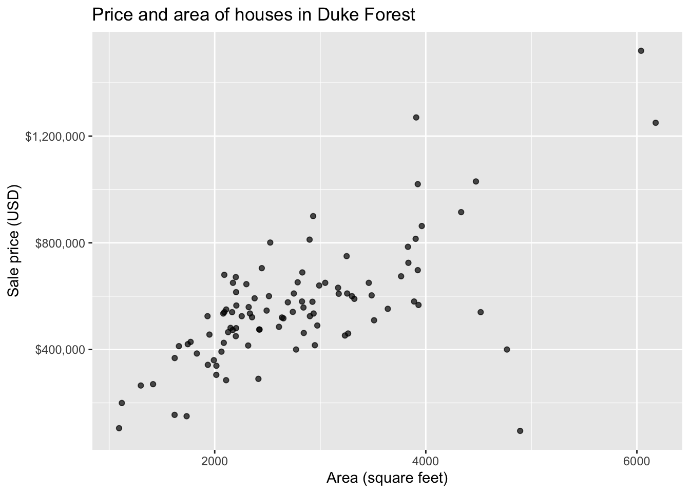
Goal: Use the area (in square feet) to understand variability in the price of houses in Duke Forest.
Exploratory data analysis
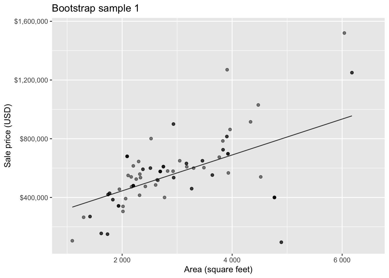
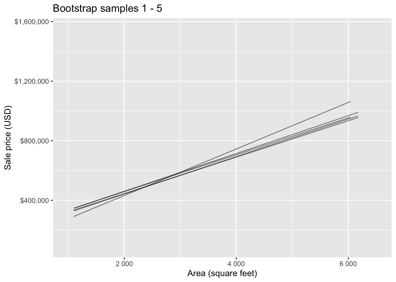
Bootstrap sample 1

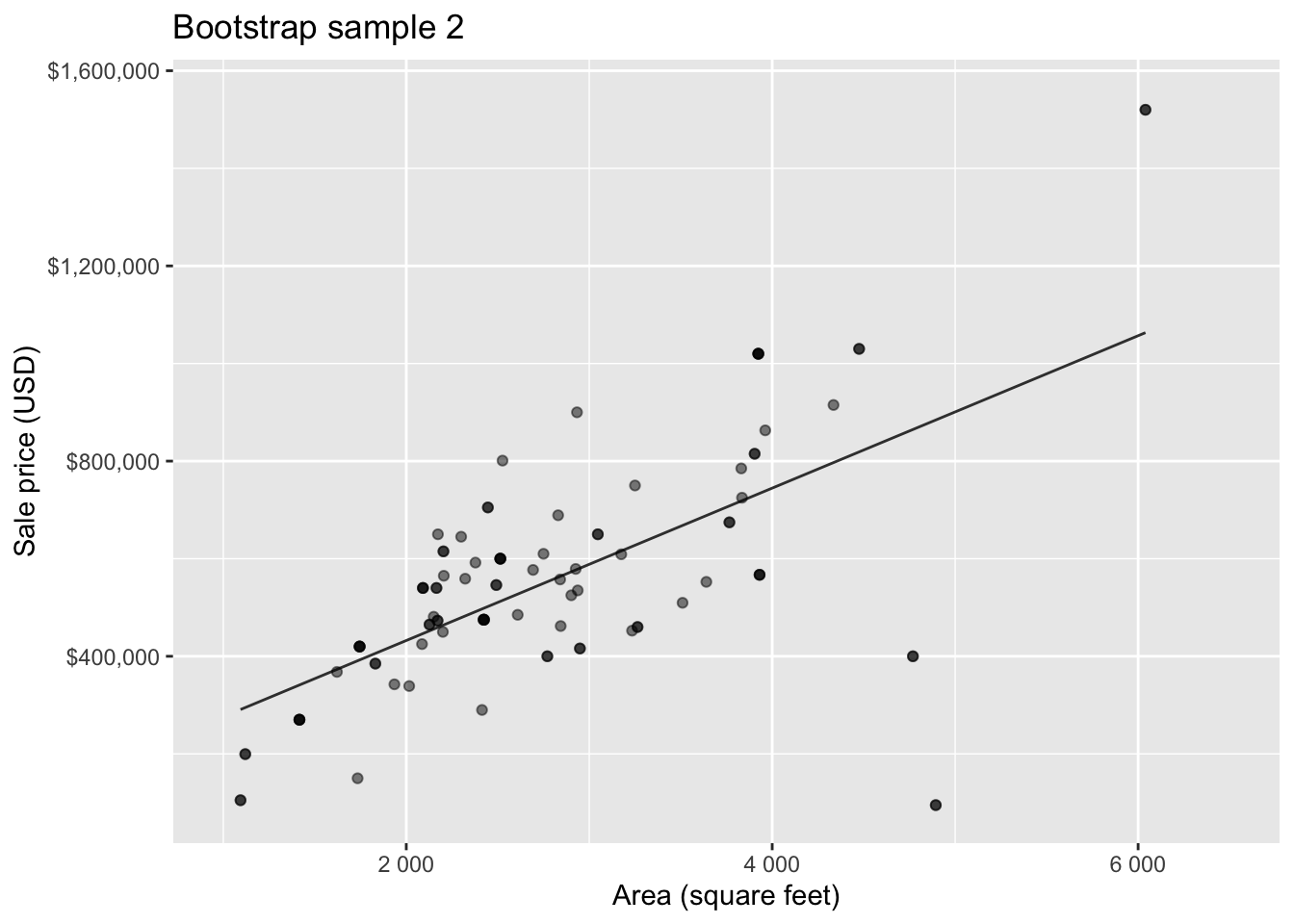
Bootstrap sample 2
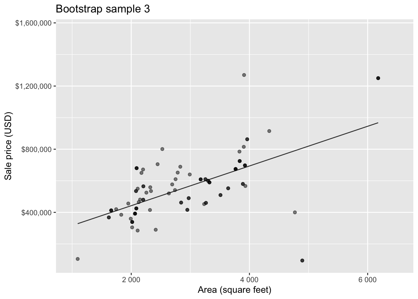
Bootstrap sample 3

Bootstrap sample 4


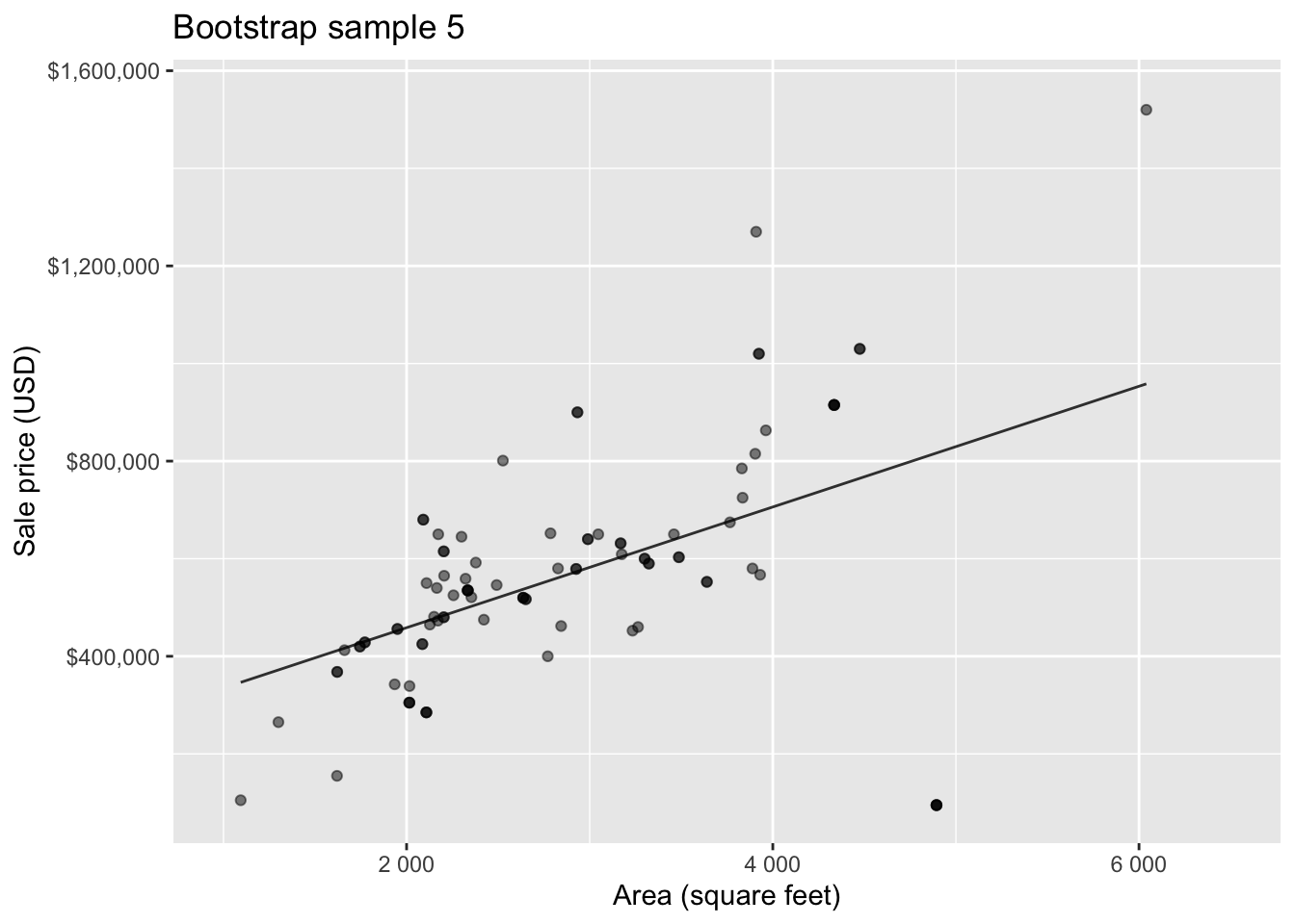
Bootstrap sample 5

so on and so forth…
Bootstrap samples 1 - 5

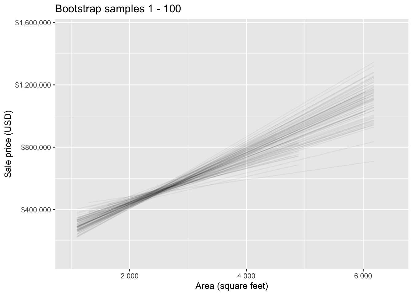
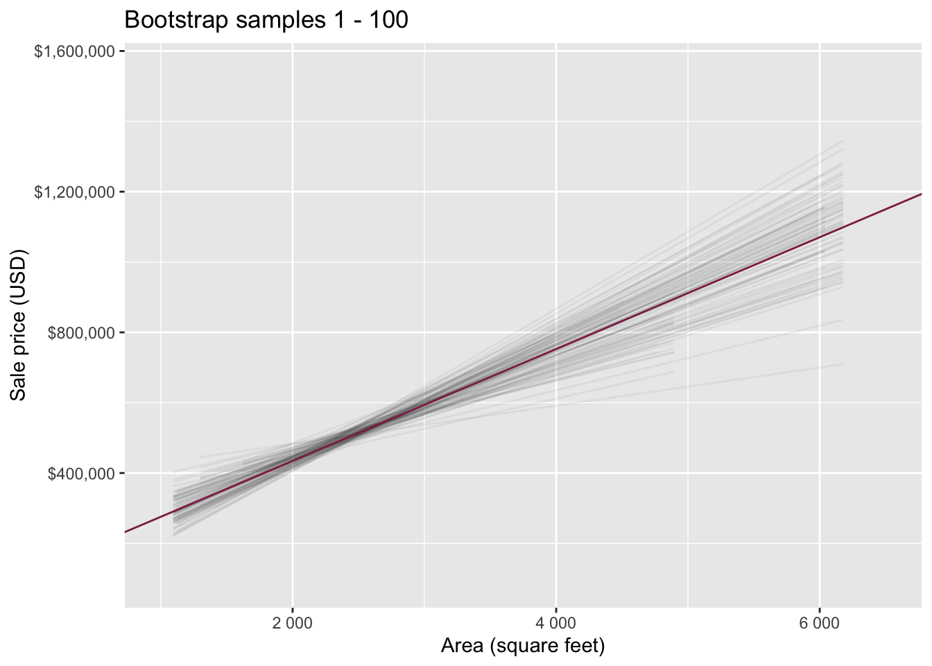
Bootstrap samples 1 - 100

Slopes of bootstrap samples
Fill in the blank: For each additional square foot, the model predicts the sale price of Duke Forest houses to be higher, on average, by $159, plus or minus ___ dollars.
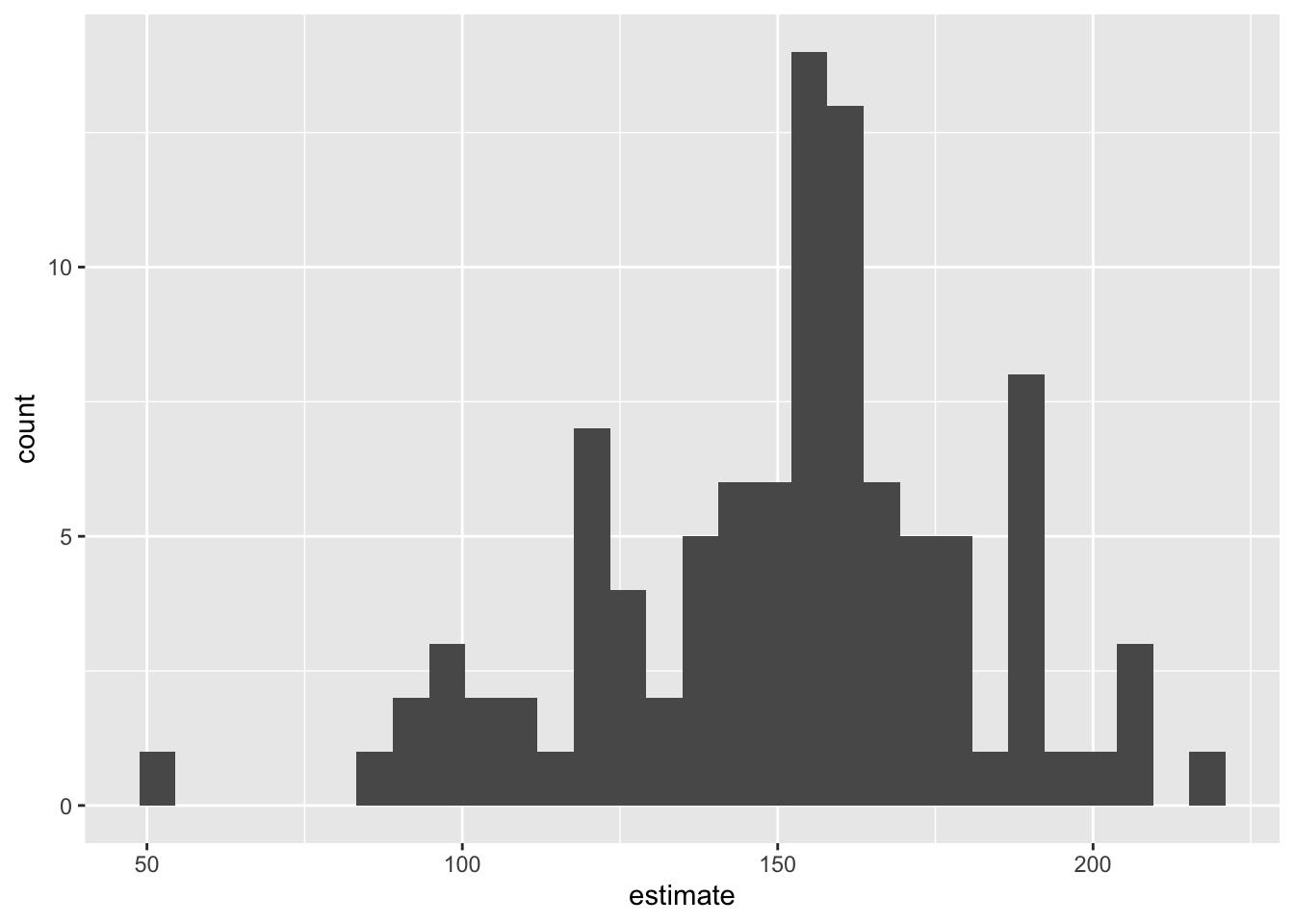
Slopes of bootstrap samples
Fill in the blank: For each additional square foot, we expect the sale price of Duke Forest houses to be higher, on average, by $159, plus or minus ___ dollars.

Confidence level
How confident are you that the true slope is between $0 and $250? How about $150 and $170? How about $90 and $210?
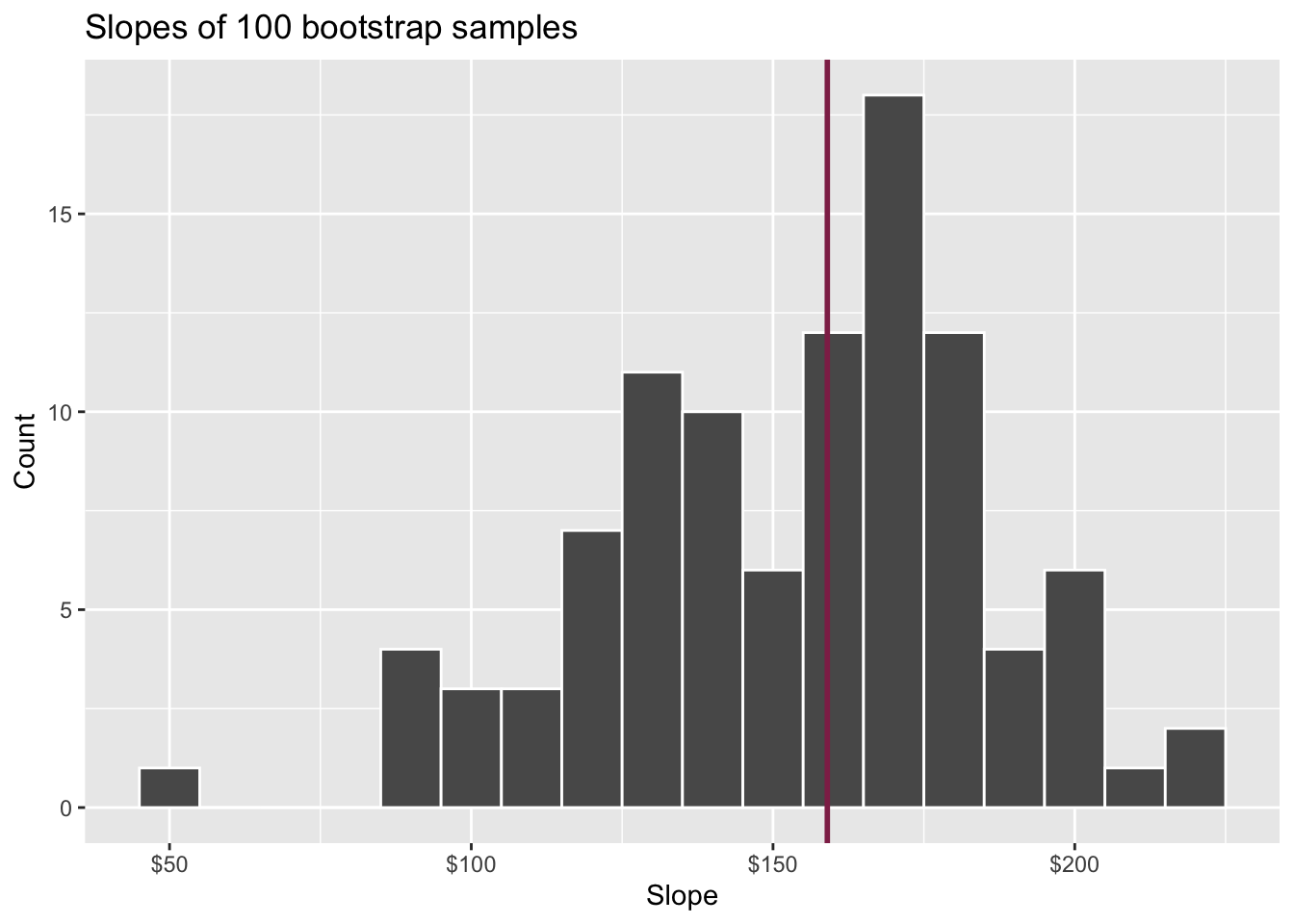
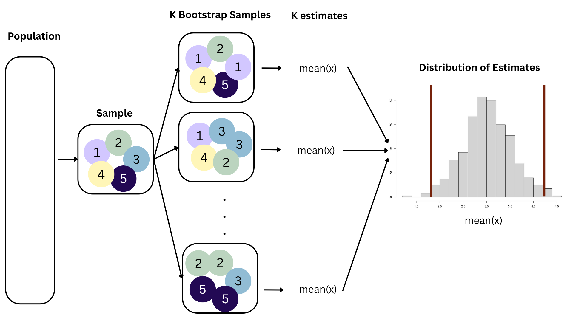
95% confidence interval
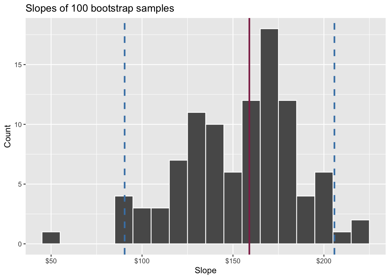
- A 95% confidence interval is bounded by the middle 95% of the bootstrap distribution
- We are 95% confident that for each additional square foot, the model predicts the sale price of Duke Forest houses to be higher, on average, by $90.43 to $205.77.
Examine bootstrap samples
Precision vs. accuracy
If we want to be very certain that we capture the population parameter, should we use a wider or a narrower interval? What drawbacks are associated with using a wider interval?