The Language of Models

Lecture 13

Published

June 4, 2025

While you wait…

Go to your ae project in RStudio.
Make sure all of your changes up to this point are committed and pushed, i.e., there’s nothing left in your Git pane.
Click Pull to get today’s application exercise file: ae-11-modeling-fish.qmd.
Wait till the you’re prompted to work on the application exercise during class before editing the file.

Announcements

No office hours today
Lab Thursday: Project proposals/identifying data sets of interest.

Midterm 1 is done!

The class is halfway over!

Before:

Plotting and summary statistics
Useful, but… a little subjective?

Now:

Learn statistical tools for quantifying relationships
- Describing relationships
- Prediction and classification
- Uncertainty quantification

Prediction / classification

Goals

What is a model?
Why do we model?
What is correlation?

Let’s drive a Tesla!

Semi or garage?

i love how Tesla thinks the wall in my garage is a semi. 😅

Source: Reddit

Semi or garage?

New owner here. Just parked in my garage. Tesla thinks I crashed onto a semi.

Source: Reddit

Car or trash?

Tesla calls Mercedes trash

Source: Reddit

Description

Leisure, commute, physical activity and BP

Relation Between Leisure Time, Commuting, and Occupational Physical Activity With Blood Pressure in 125,402 Adults: The Lifelines Cohort

Byambasukh, Oyuntugs, Harold Snieder, and Eva Corpeleijn. “Relation between leisure time, commuting, and occupational physical activity with blood pressure in 125 402 adults: the lifelines cohort.” Journal of the American Heart Association 9.4 (2020): e014313.

Leisure, commute, physical activity and BP

Goal: To investigate the associations of different domains of daily‐life physical activity, such as commuting, leisure‐time, and occupational, with BP level and the risk of having hypertension.

Leisure, commute, physical activity and BP

Goal: To investigate the associations of different domains of daily-life physical activity, such as commuting, leisure-time, and occupational, with BP level and the risk of having hypertension.

Leisure, commute, physical activity and BP

Goal: To investigate the associations of different domains of daily-life physical activity, such as commuting, leisure-time, and occupational, with BP level and the risk of having hypertension.

Leisure, commute, physical activity and BP

Goal: To investigate the associations of different domains of daily-life physical activity, such as commuting, leisure-time, and occupational, with BP level and the risk of having hypertension.

Methods and Results: In the population-based Lifelines cohort (N=125,402), MVPA was assessed by the Short Questionnaire to Assess Health-Enhancing Physical Activity, a validated questionnaire in different domains such as commuting, leisure-time, and occupational PA. Commuting-and-leisure-time MVPA was associated with BP in a dose-dependent manner. β Coefficients (95% CI) from linear regression analyses were −1.64 (−2.03 to −1.24), −2.29 (−2.68 to −1.90), and −2.90 (−3.29 to −2.50) mm Hg systolic BP for the low, middle, and highest tertile of MVPA compared with “No MVPA” as the reference group after adjusting for age, sex, education, smoking and alcohol use. Further adjustment for body mass index attenuated the associations by 30% to 50%, but more MVPA remained significantly associated with lower BP and lower risk of hypertension. This association was age dependent. β Coefficients (95% CI) for the highest tertiles of commuting-and-leisure-time MVPA were −1.67 (−2.20 to −1.15), −3.39 (−3.94 to −2.82) and −4.64 (−6.15 to −3.14) mm Hg systolic BP in adults <40, 40 to 60, and >60 years, respectively.

Leisure, commute, physical activity and BP

Goal: To investigate the associations of different domains of daily-life physical activity, such as commuting, leisure-time, and occupational, with BP level and the risk of having hypertension.

Conclusions: Higher commuting and leisure-time but not occupational MVPA were significantly associated with lower BP and lower hypertension risk at all ages, but these associations were stronger in older adults.

Modeling

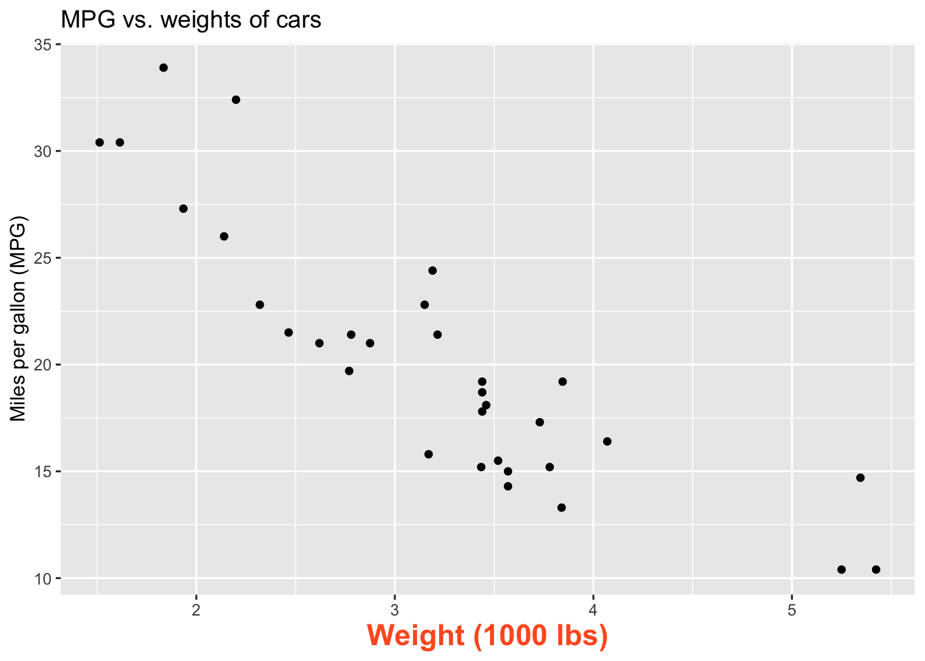
Modeling cars

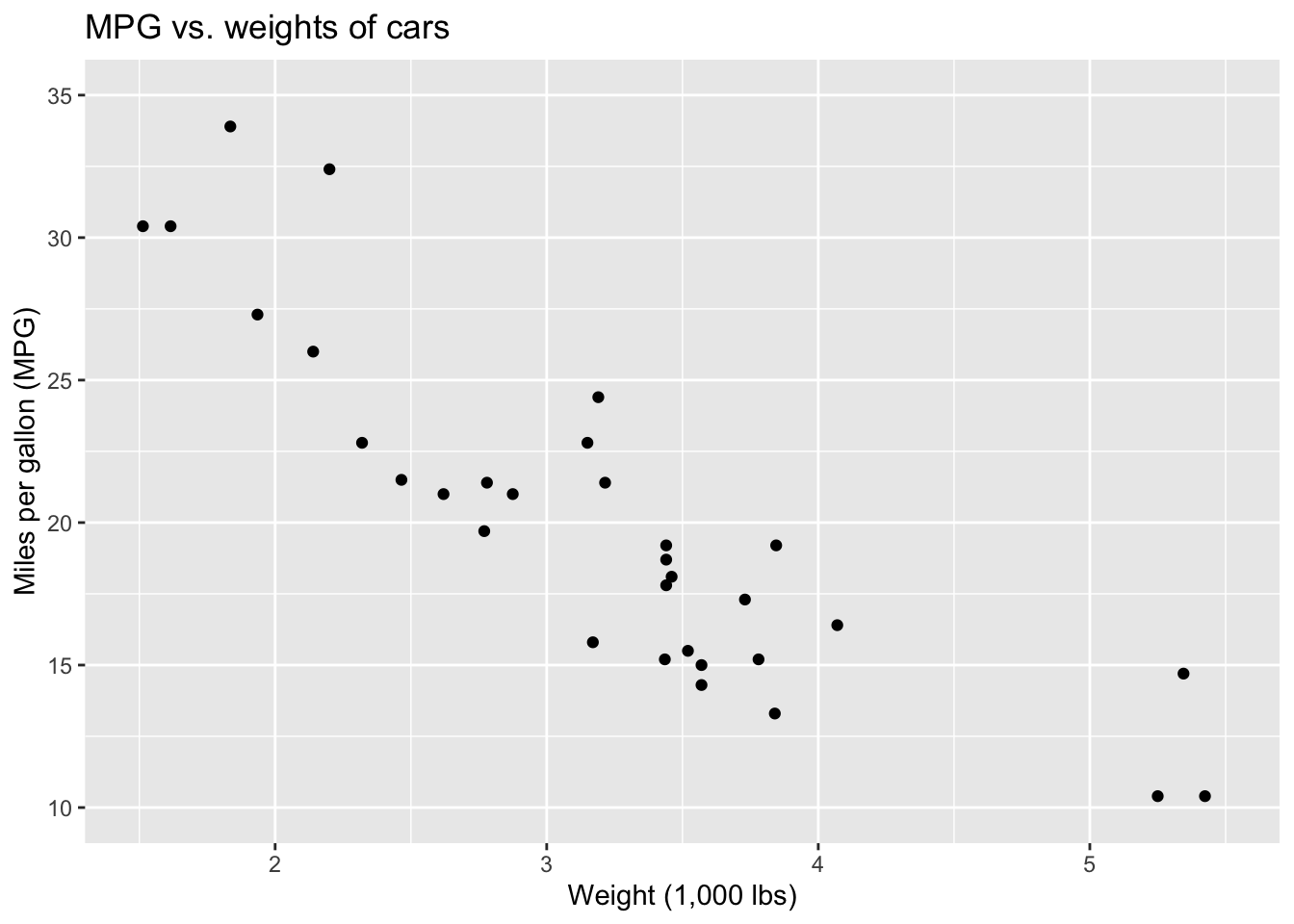
What is the relationship between cars’ weights and their mileage?
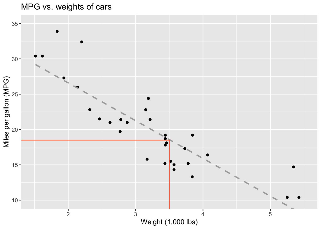
What is your best guess for a car’s MPG that weighs 3,500 pounds?

Modelling cars

Describe: What is the relationship between cars’ weights and their mileage?

Modelling cars

Predict: What is your best guess for a car’s MPG that weighs 3,500 pounds?

Modelling

Use models to explain the relationship between variables and to make predictions
For now we will focus on linear models (but there are many many other types of models too!)

What is a line?

But on a plot…

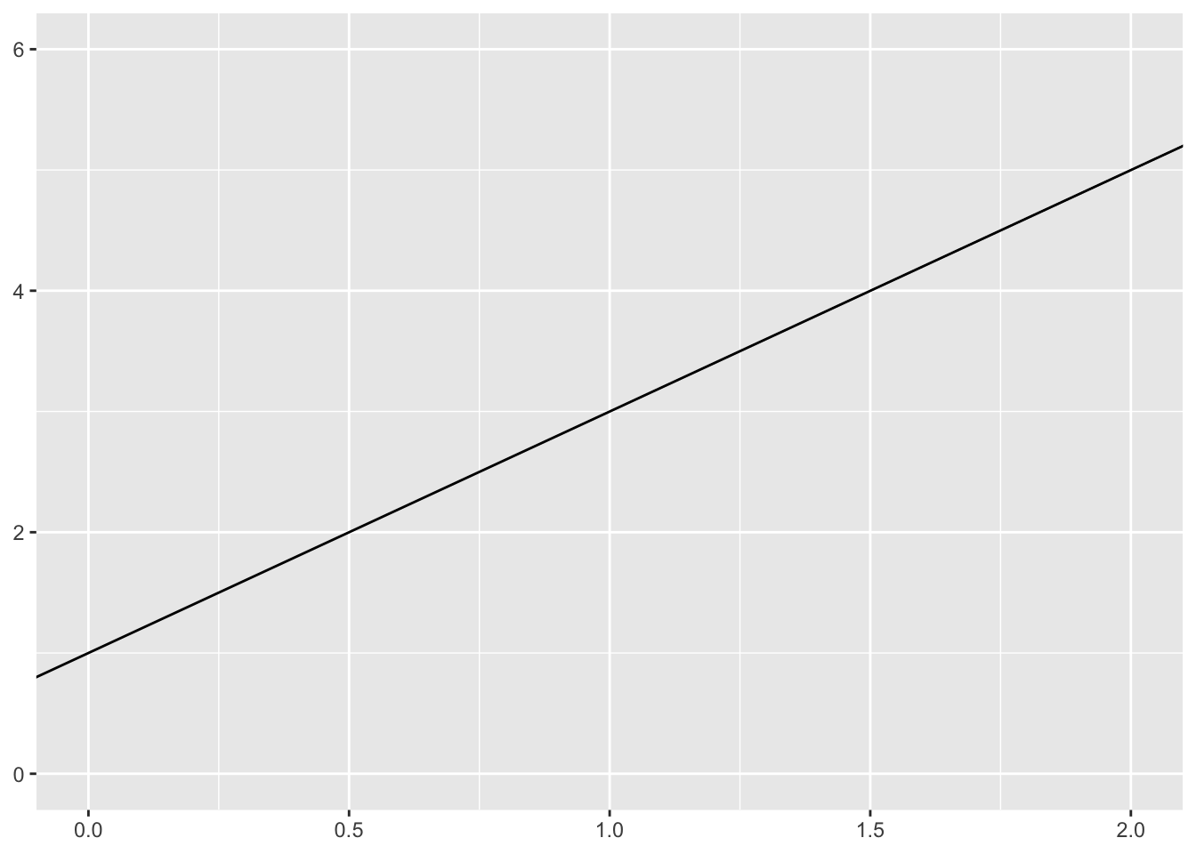
But in math terms…

\[ y = mx + b \]

Modelling vocabulary

Predictor (explanatory variable)
Outcome (response variable)
Regression line
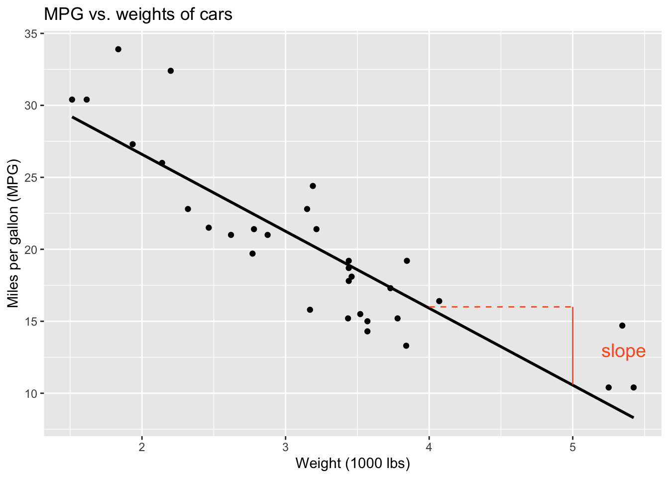
- Slope
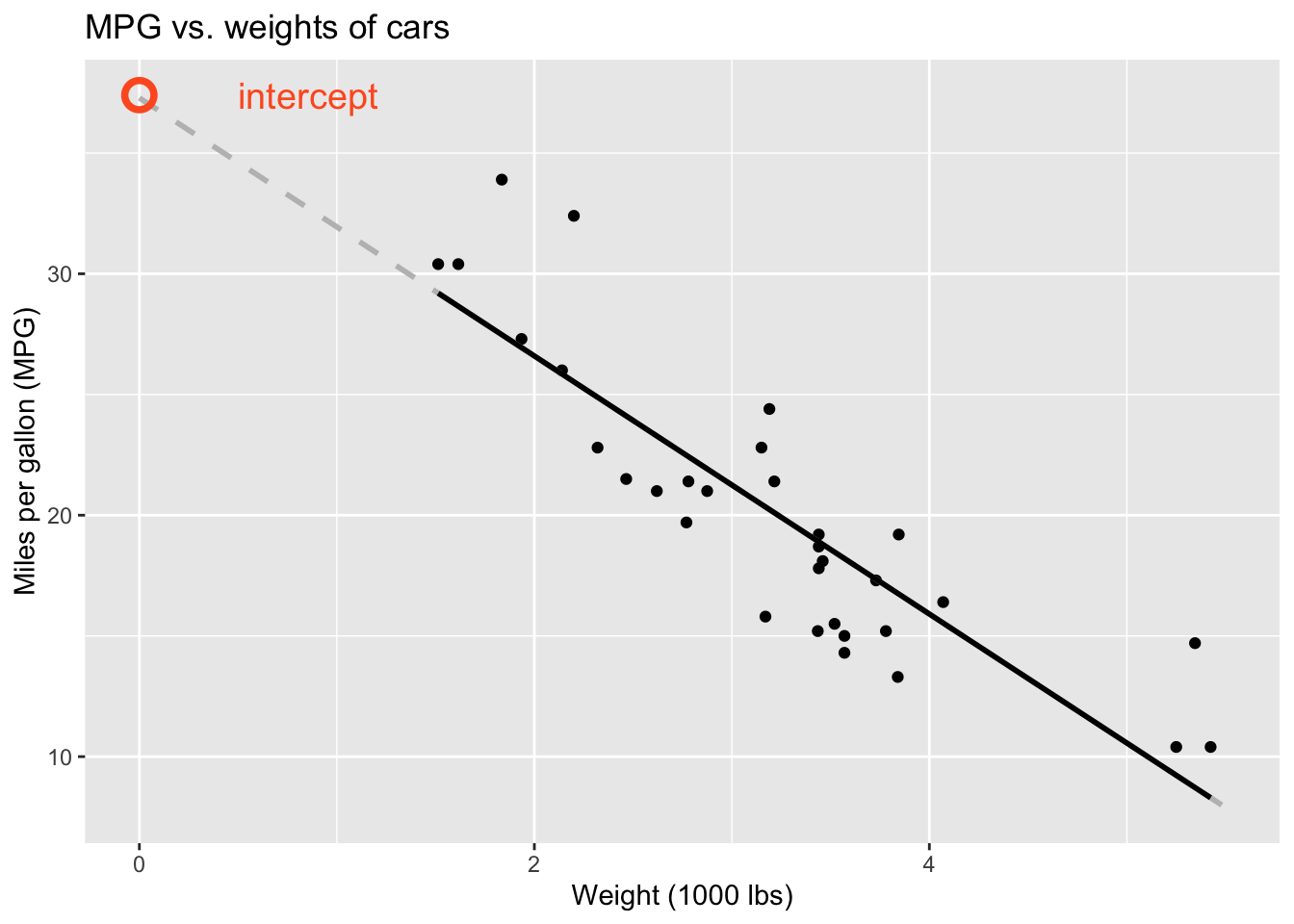
- Intercept
Correlation

Predictor (explanatory variable)

mpg	wt
21	2.62
21	2.875
22.8	2.32
21.4	3.215
18.7	3.44
18.1	3.46
...	...

Outcome (response variable)

mpg	wt
21	2.62
21	2.875
22.8	2.32
21.4	3.215
18.7	3.44
18.1	3.46
...	...

Regression line

Regression line: slope

Regression line: intercept

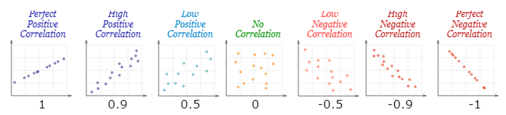
Correlation

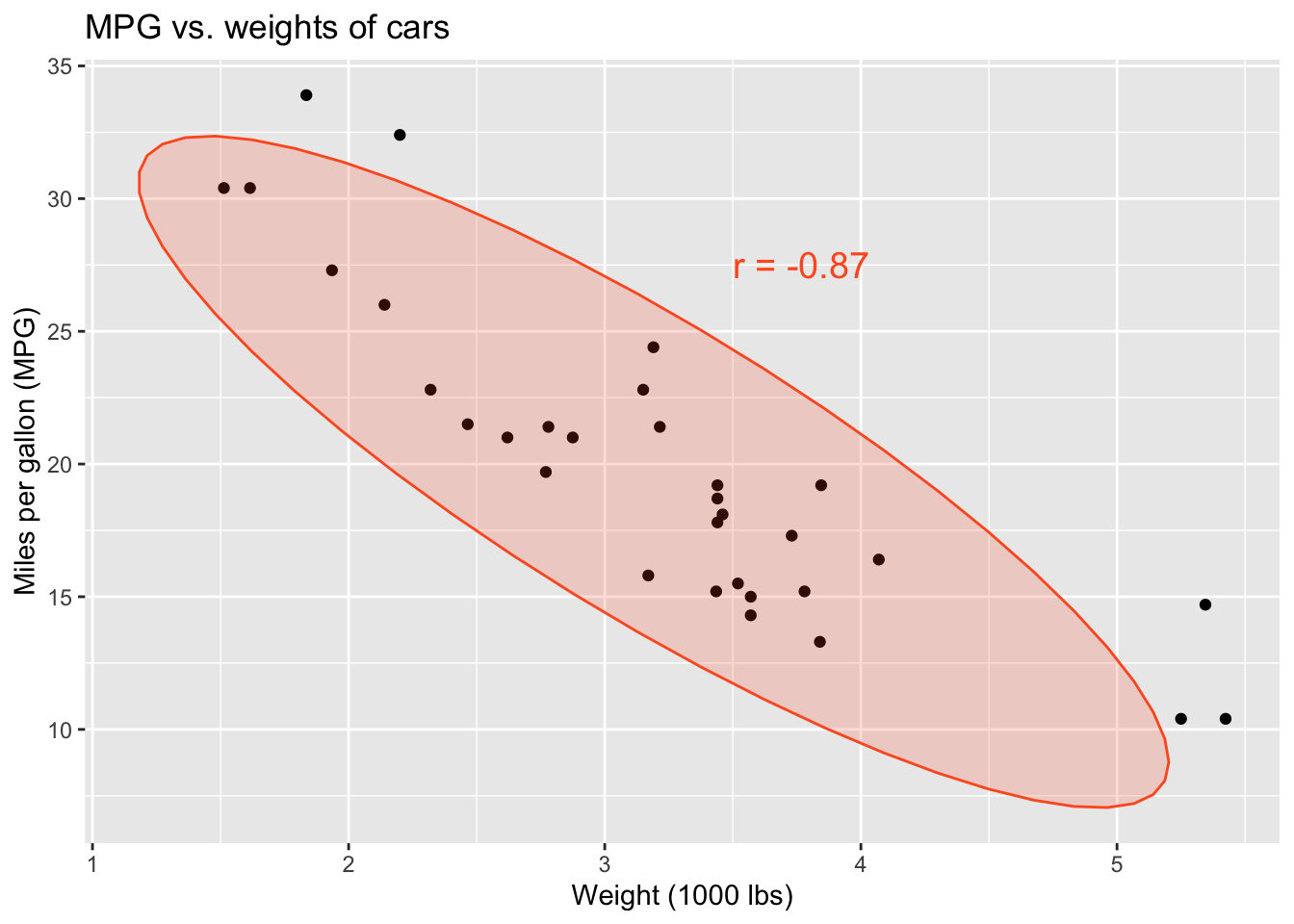
Correlation

Ranges between -1 and 1.
Same sign as the slope.

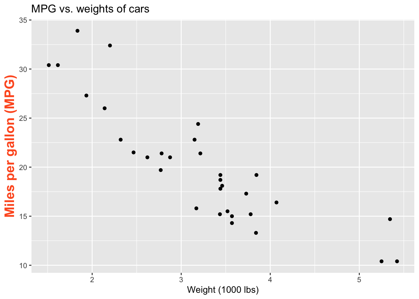
Visualizing the model

ggplot(mtcars, aes(x = wt, y = mpg)) +
  geom_point()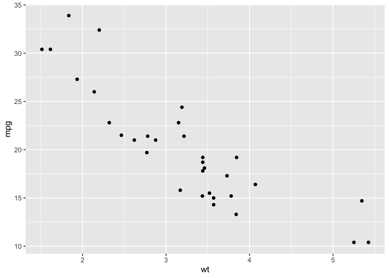

Visualizing the model

ggplot(mtcars, aes(x = wt, y = mpg)) +
  geom_point() + 
  geom_smooth()

`geom_smooth()` using method = 'loess' and formula = 'y ~ x'

Visualizing the model

ggplot(mtcars, aes(x = wt, y = mpg)) +
  geom_point() + 
  geom_smooth(method = "loess")

`geom_smooth()` using formula = 'y ~ x'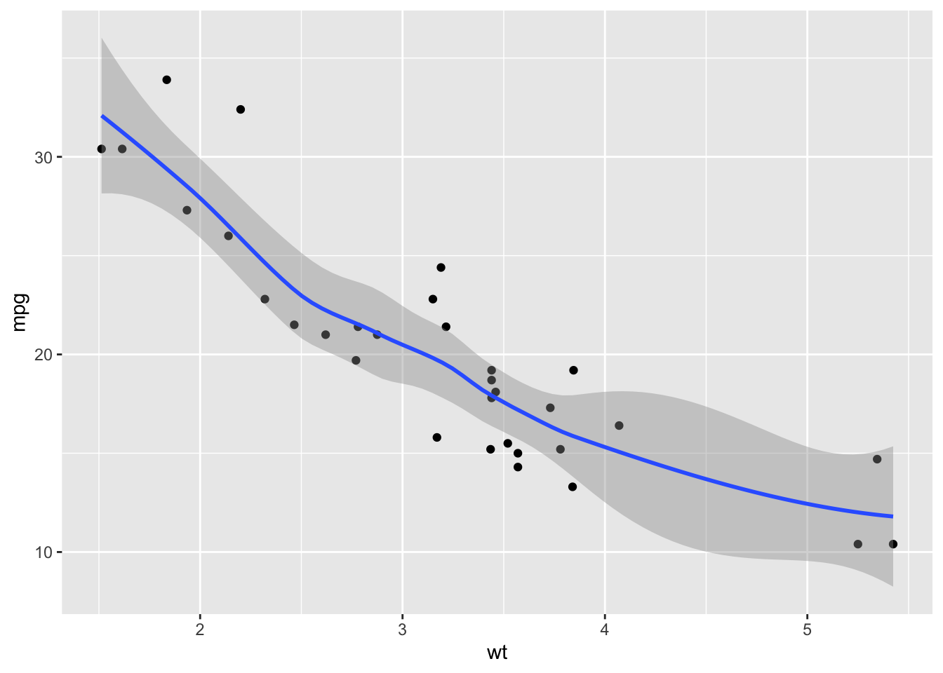

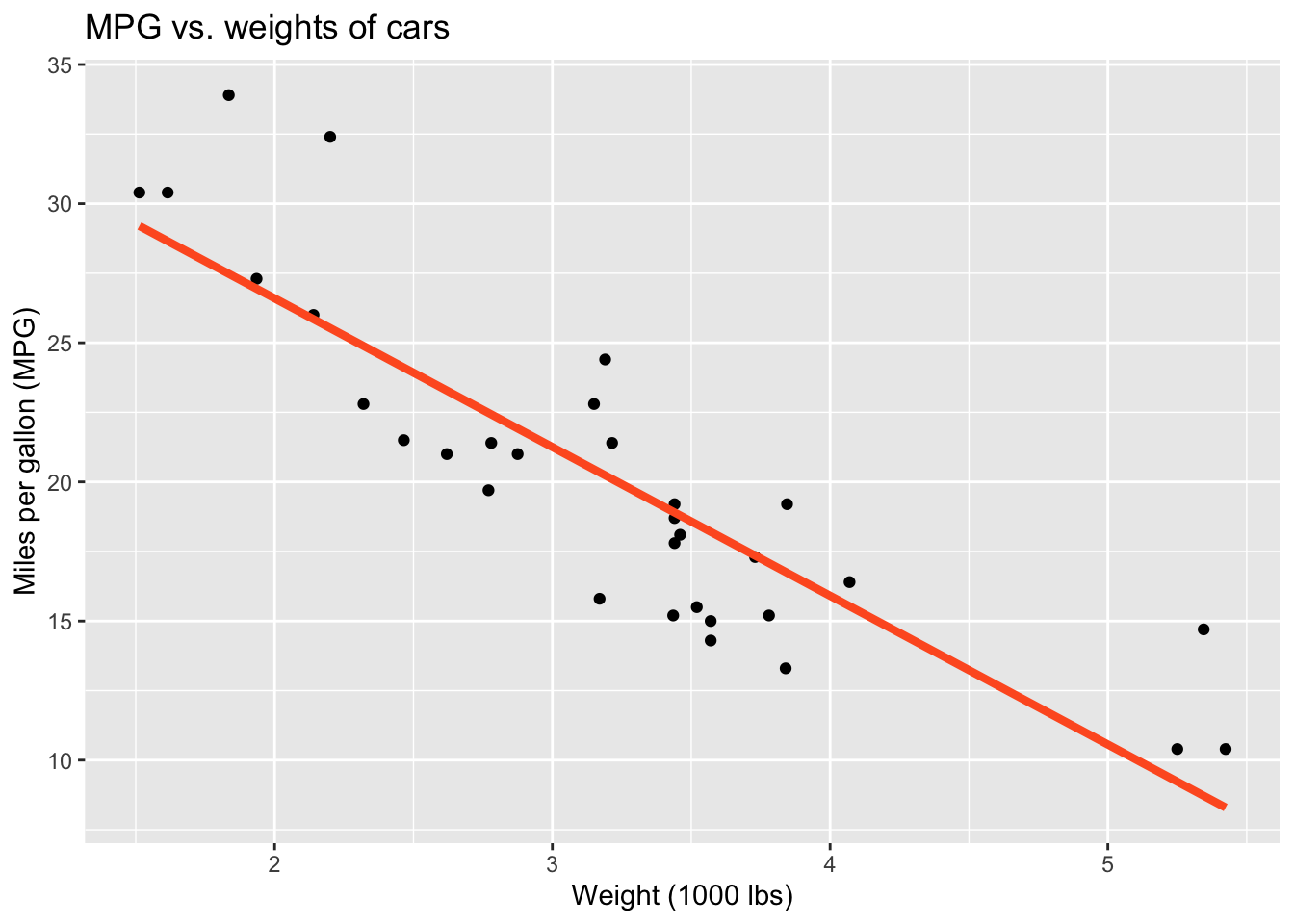
Visualizing the model

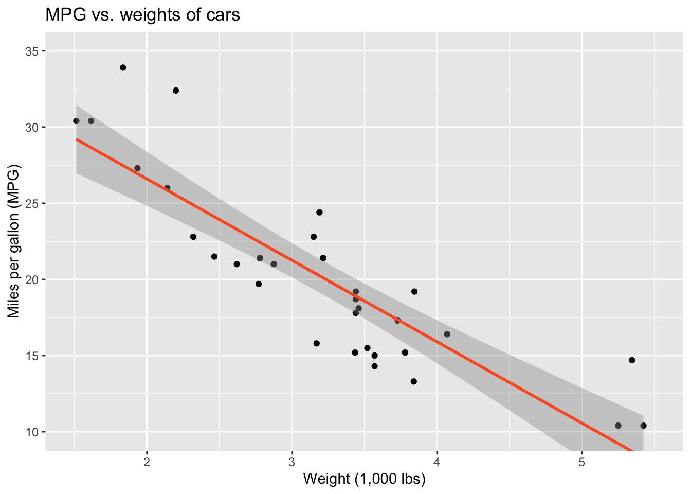
ggplot(mtcars, aes(x = wt, y = mpg)) +
  geom_point() + 
  geom_smooth(method = "lm")

`geom_smooth()` using formula = 'y ~ x'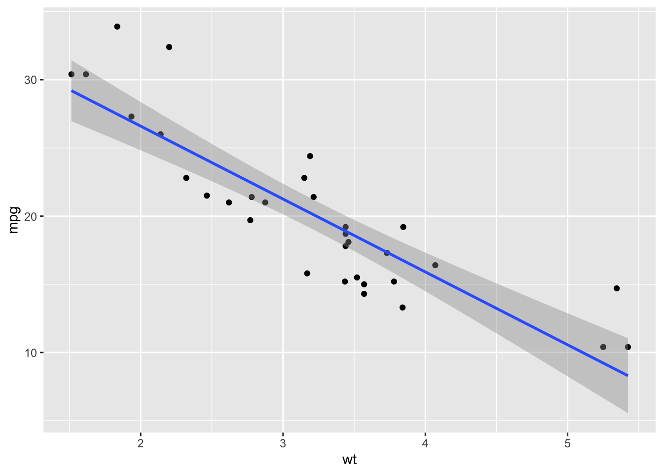

Application exercise

Follow along

ae-11-modeling-fish

Go to your ae project in RStudio.
If you haven’t yet done so, make sure all of your changes up to this point are committed and pushed, i.e., there’s nothing left in your Git pane.
If you haven’t yet done so, click Pull to get today’s application exercise file: ae-11-modeling-fish.qmd.
Work through the application exercise in class, and render, commit, and push your edits.

Data: Fish

library(tidyverse)
library(tidymodels)

fish <- read_csv("data/fish.csv")

Data: Fish

fish

# A tibble: 55 × 7
   species weight length_vertical length_diagonal length_cross height
   <chr>    <dbl>           <dbl>           <dbl>        <dbl>  <dbl>
 1 Bream      242            23.2            25.4         30     11.5
 2 Bream      290            24              26.3         31.2   12.5
 3 Bream      340            23.9            26.5         31.1   12.4
 4 Bream      363            26.3            29           33.5   12.7
 5 Bream      430            26.5            29           34     12.4
 6 Bream      450            26.8            29.7         34.7   13.6
 7 Bream      500            26.8            29.7         34.5   14.2
 8 Bream      390            27.6            30           35     12.7
 9 Bream      450            27.6            30           35.1   14.0
10 Bream      500            28.5            30.7         36.2   14.2
# ℹ 45 more rows
# ℹ 1 more variable: width <dbl>

Visualizing the model

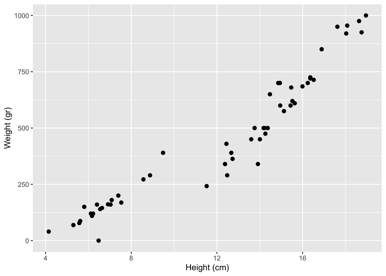
Goal: Analyze the relationship between fish height and weight.

Visualizing the model

Goal: Analyze the relationship between fish height and weight.

ggplot(fish, aes(x = height,
                 y = weight)) +
  geom_point() +
  labs(x = "Height (cm)",
       y = "Weight (gr)")

Visualizing the model

Goal: Analyze the relationship between fish height and weight.

Where would you draw a line?

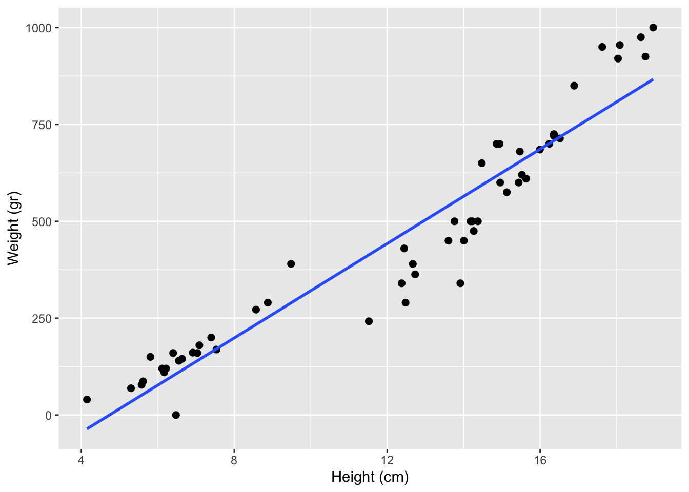
Visualizing the model

Let R draw the line for you!

ggplot(fish, aes(x = height,
                 y = weight)) +
  geom_point() +
  geom_smooth(method = "lm", se = FALSE) +
  labs(x = "Height (cm)",
       y = "Weight (gr)")

Visualizing the model

How can we use the line to make predictions?

Predict weight given height:

10 cm
15 cm
20 cm

Visualizing the model

Are the predictions good?

Residual: Difference between observed and predicted value

Model Fitting

Fit your first model

fish_hw_fit <- linear_reg() |>
  fit(weight ~ height, data = fish)

Fit your first model

fish_hw_fit <- linear_reg() |>
  fit(weight ~ height, data = fish)

fish_hw_fit

parsnip model object


Call:
stats::lm(formula = weight ~ height, data = data)

Coefficients:
(Intercept)       height  
    -288.42        60.92

Model prediction

Use model results to predict weights at heights 10cm, 15cm, and 20cm.

fish_hw_fit

parsnip model object


Call:
stats::lm(formula = weight ~ height, data = data)

Coefficients:
(Intercept)       height  
    -288.42        60.92

x <- 10
-288 + 60.92 * x

[1] 321.2

Model prediction: full data

Goal: Calculate predicted weights for all fish in the data.

fish_hw_aug <- augment(fish_hw_fit, new_data = fish)

Model prediction: full data

Goal: Calculate predicted weights for all fish in the data.

fish_hw_aug <- augment(fish_hw_fit, new_data = fish)
fish_hw_aug

# A tibble: 55 × 9
   .pred .resid species weight height length_vertical length_diagonal
   <dbl>  <dbl> <chr>    <dbl>  <dbl>           <dbl>           <dbl>
 1  413. -171.  Bream      242   11.5            23.2            25.4
 2  472. -182.  Bream      290   12.5            24              26.3
 3  466. -126.  Bream      340   12.4            23.9            26.5
 4  487. -124.  Bream      363   12.7            26.3            29  
 5  470.  -39.6 Bream      430   12.4            26.5            29  
 6  540.  -90.2 Bream      450   13.6            26.8            29.7
 7  575.  -75.3 Bream      500   14.2            26.8            29.7
 8  483.  -93.4 Bream      390   12.7            27.6            30  
 9  565. -115.  Bream      450   14.0            27.6            30  
10  578.  -78.2 Bream      500   14.2            28.5            30.7
# ℹ 45 more rows
# ℹ 2 more variables: length_cross <dbl>, width <dbl>

Model evaluation: residuals

Goal: Visualize the residuals

fish_hw_aug |> 
  ggplot(aes(x = height,
             y = weight)) + 
  geom_point() + 
  geom_smooth(method = "lm", 
              se = FALSE) +
  theme_minimal()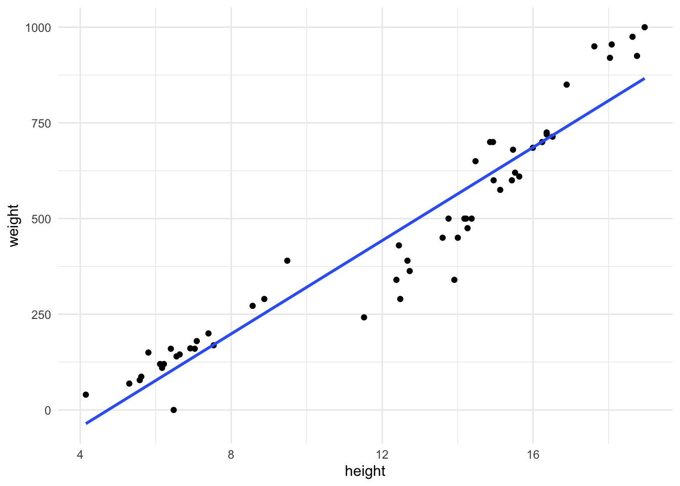

Model evaluation: residuals

Goal: Visualize the residuals

fish_hw_aug |> 
  ggplot(aes(x = height,
             y = weight)) + 
  geom_point() + 
  geom_smooth(method = "lm", 
              se = FALSE) +
  geom_segment(aes(xend = height, 
                   yend = .pred)) +
  theme_minimal()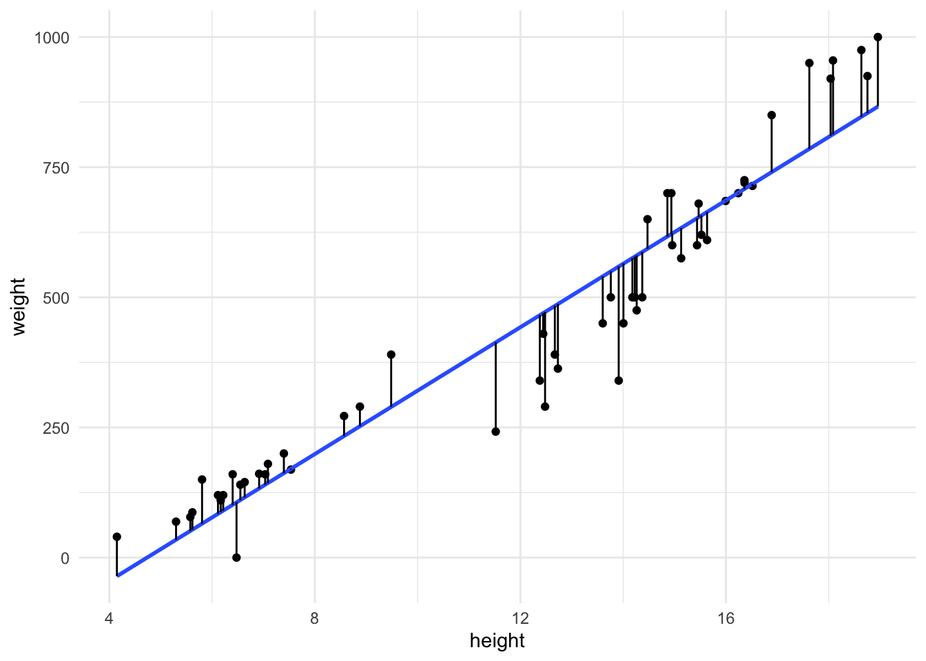

Model Summary

fish_hw_fit

parsnip model object


Call:
stats::lm(formula = weight ~ height, data = data)

Coefficients:
(Intercept)       height  
    -288.42        60.92

fish_hw_tidy <- tidy(fish_hw_fit)
fish_hw_tidy

# A tibble: 2 × 5
  term        estimate std.error statistic  p.value
  <chr>          <dbl>     <dbl>     <dbl>    <dbl>
1 (Intercept)   -288.      34.0      -8.49 1.83e-11
2 height          60.9      2.64     23.1  2.40e-29

Correlation

Strength and direction of a linear relationship. It’s bounded by -1 and 1.

Correlation

fish |>
  summarize(r = cor(height, weight))

# A tibble: 1 × 1
      r
  <dbl>
1 0.954

Adding a 3rd Variable

Does the relationship between heights and weights of fish change if we take into consideration species?

ggplot(fish, 
       aes(x = height, y = weight, color = species)) +
  geom_point() +
  geom_smooth(method = "lm") +
  labs(
    title = "Weights vs. heights of fish",
    x = "Height (cm)",
    y = "Weight (gr)"
  )

`geom_smooth()` using formula = 'y ~ x'

Adding a 3rd Variable

Does the relationship between heights and weights of fish change if we take into consideration species?

ggplot(fish, 
       aes(x = height, y = weight, color = species)) +
  geom_point() +
  geom_smooth(method = "lm") +
  labs(
    title = "Weights vs. heights of fish",
    x = "Height (cm)",
    y = "Weight (gr)"
  )

`geom_smooth()` using formula = 'y ~ x'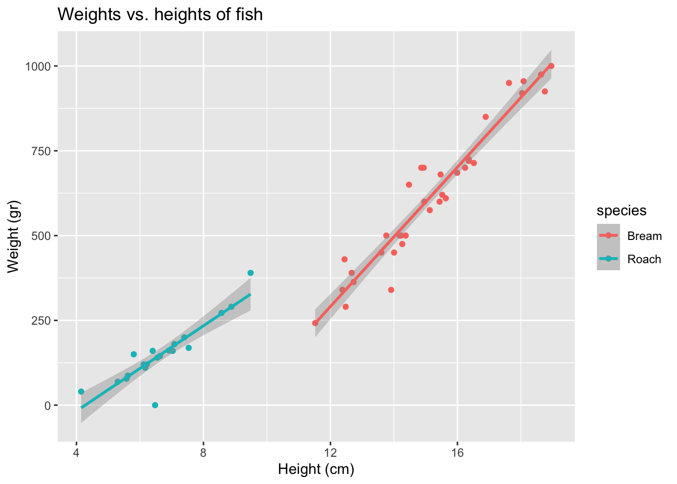