The Language of Models
Lecture 13
June 4, 2025
Semi or garage?
i love how Tesla thinks the wall in my garage is a semi. 😅
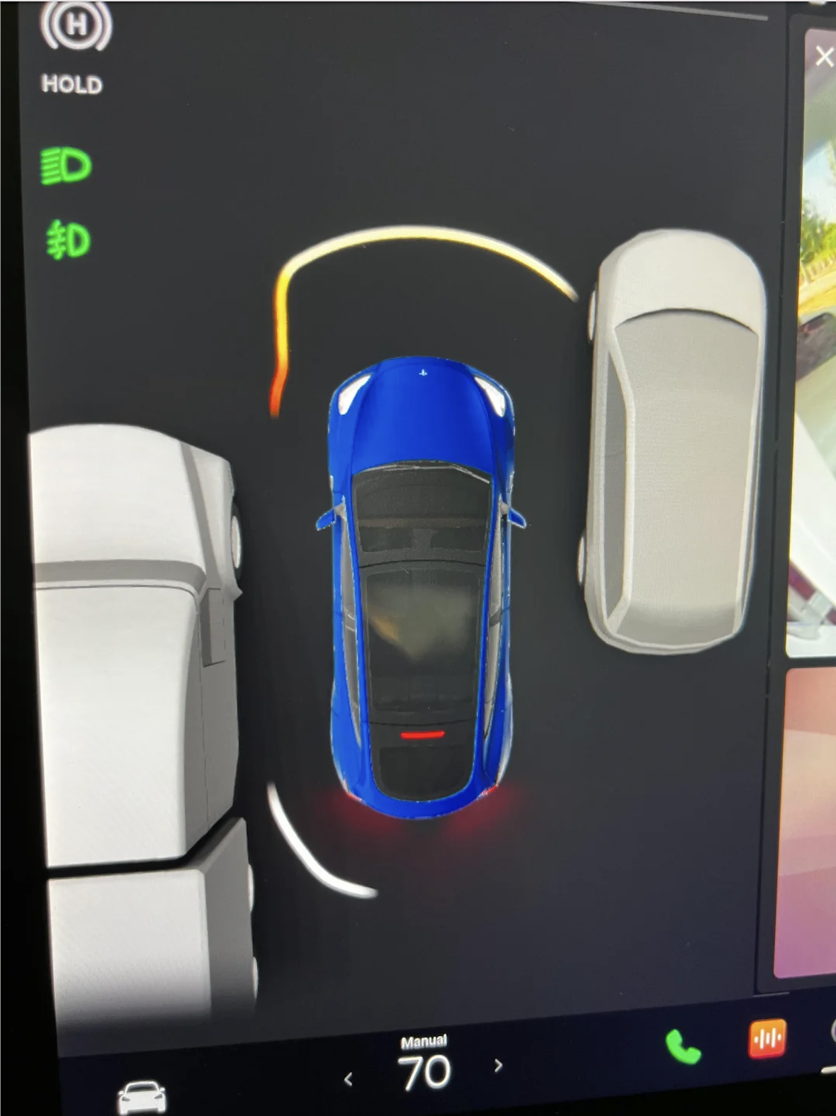
Semi or garage?
New owner here. Just parked in my garage. Tesla thinks I crashed onto a semi.

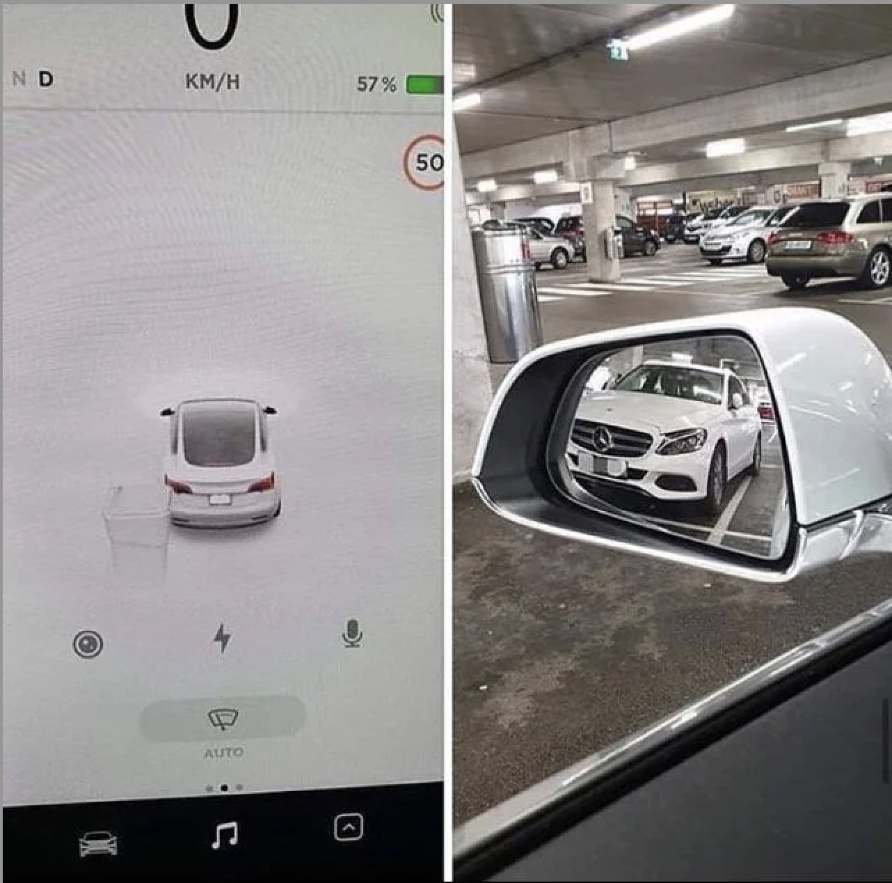
Car or trash?
Tesla calls Mercedes trash
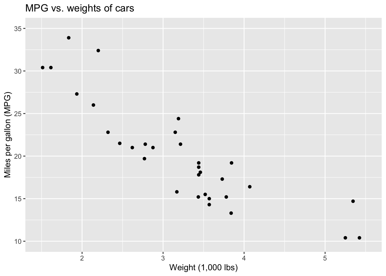
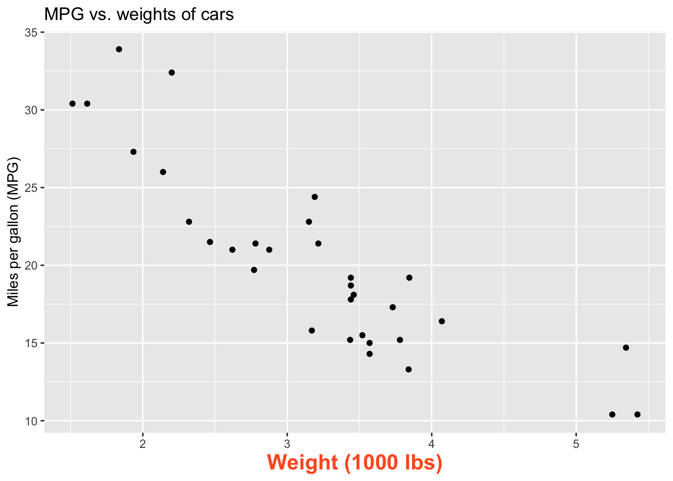
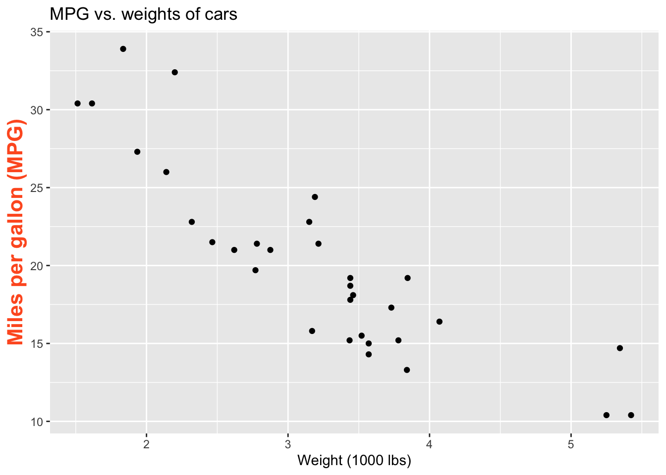
Modelling cars
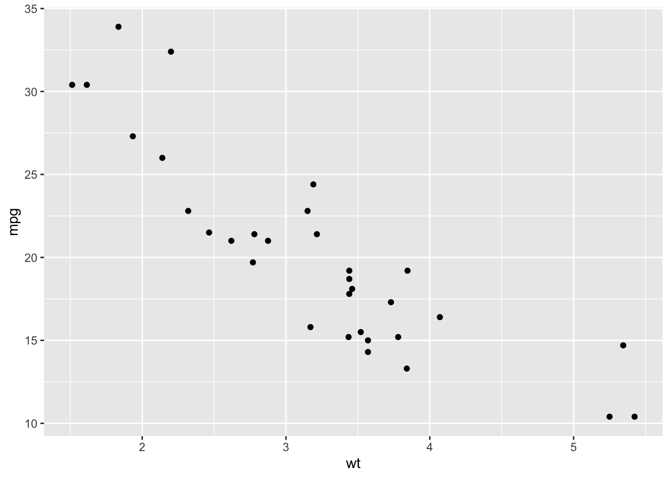
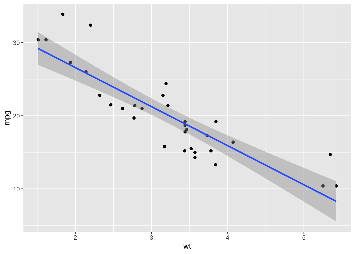
Describe: What is the relationship between cars’ weights and their mileage?
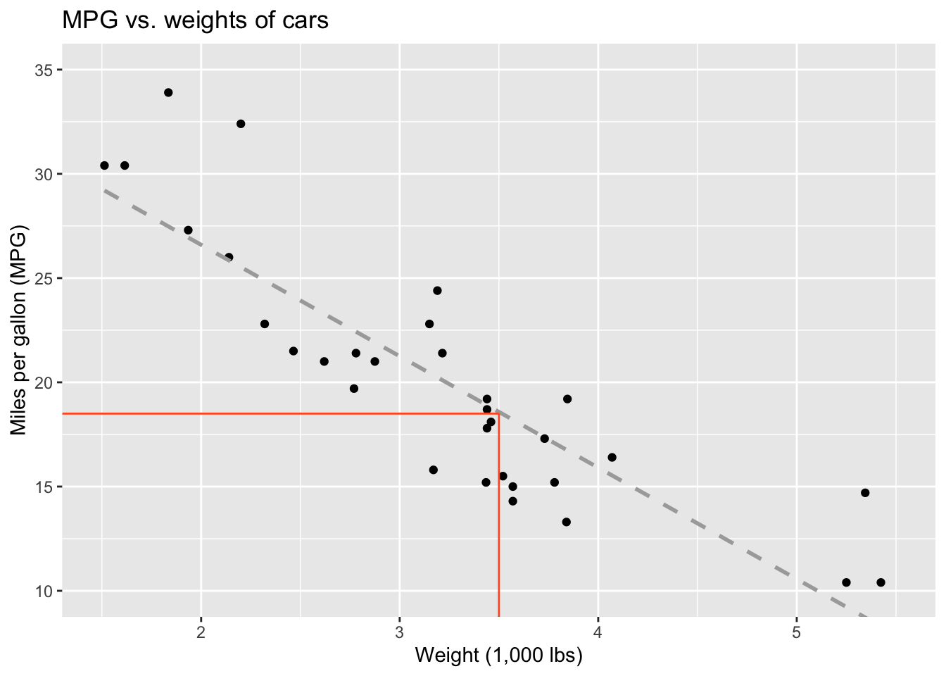
Modelling cars
Predict: What is your best guess for a car’s MPG that weighs 3,500 pounds?
What is a line?
But on a plot…
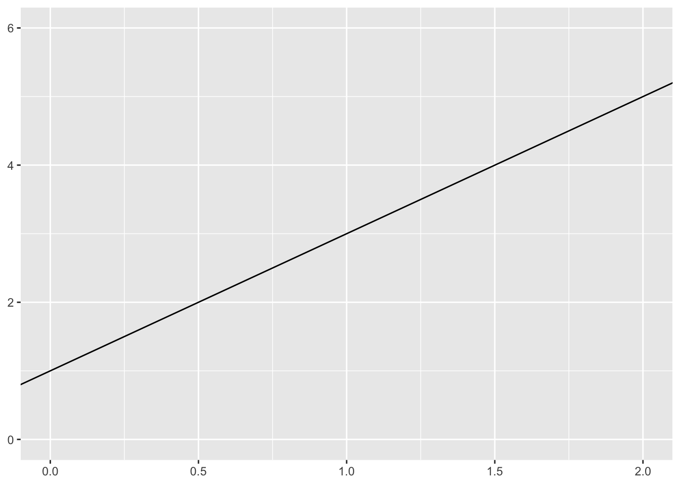
But in math terms…
\[ y = mx + b \]

Predictor (explanatory variable)
| mpg | wt |
|---|---|
| 21 | 2.62 |
| 21 | 2.875 |
| 22.8 | 2.32 |
| 21.4 | 3.215 |
| 18.7 | 3.44 |
| 18.1 | 3.46 |
| ... | ... |
Outcome (response variable)
| mpg | wt |
|---|---|
| 21 | 2.62 |
| 21 | 2.875 |
| 22.8 | 2.32 |
| 21.4 | 3.215 |
| 18.7 | 3.44 |
| 18.1 | 3.46 |
| ... | ... |
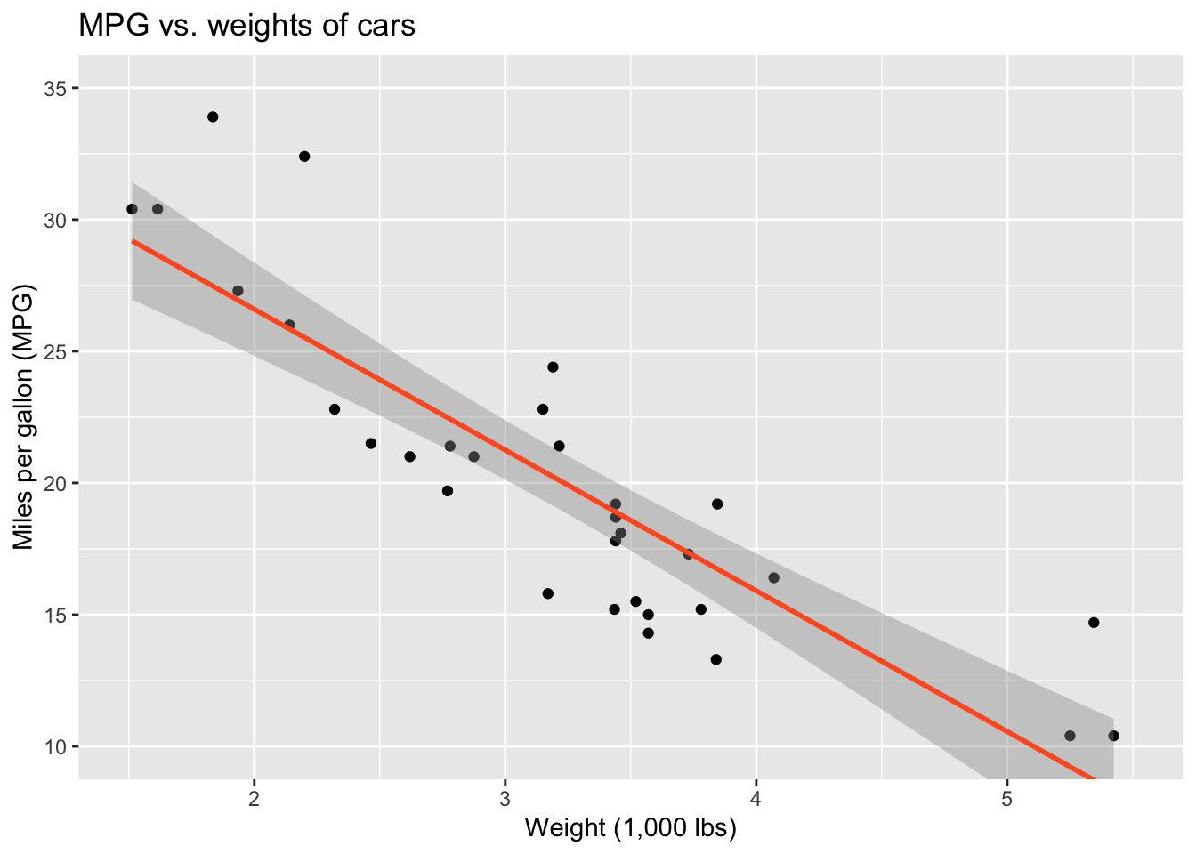
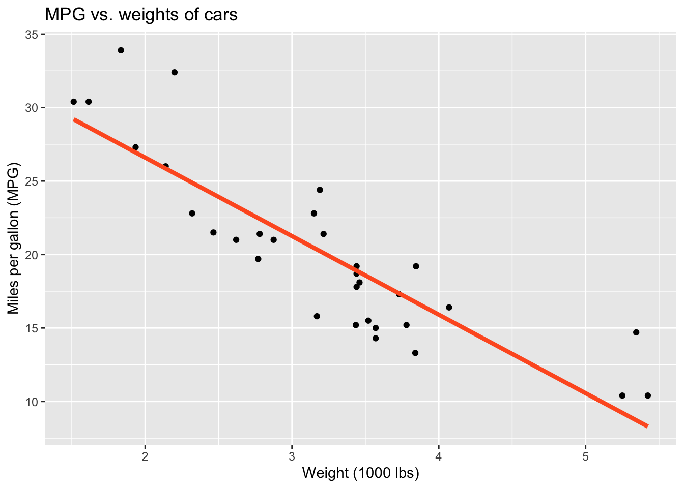
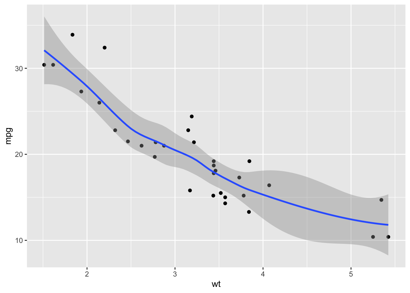
Regression line
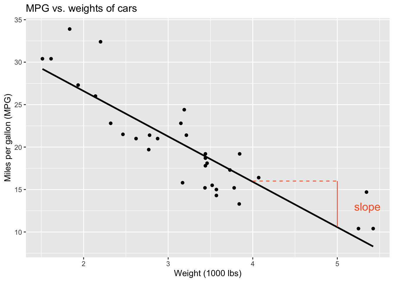
Regression line: slope
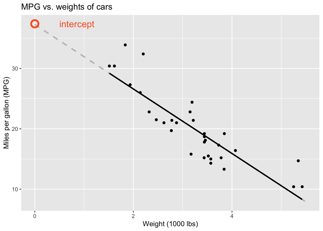
Regression line: intercept
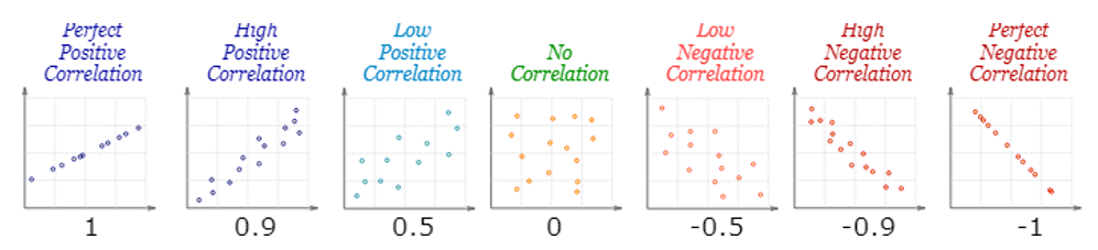
Correlation
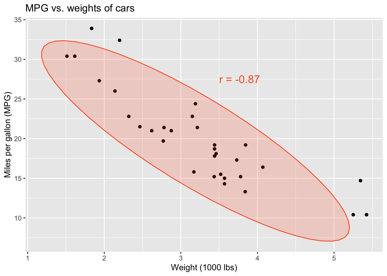
Correlation
- Ranges between -1 and 1.
- Same sign as the slope.
Visualizing the model
Visualizing the model

Visualizing the model
Visualizing the model
Visualizing the model
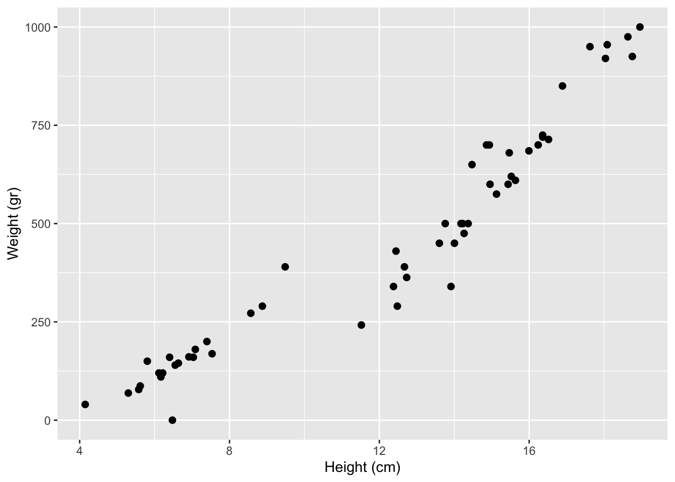
Goal: Analyze the relationship between fish height and weight.

Visualizing the model
Goal: Analyze the relationship between fish height and weight.
Where would you draw a line?
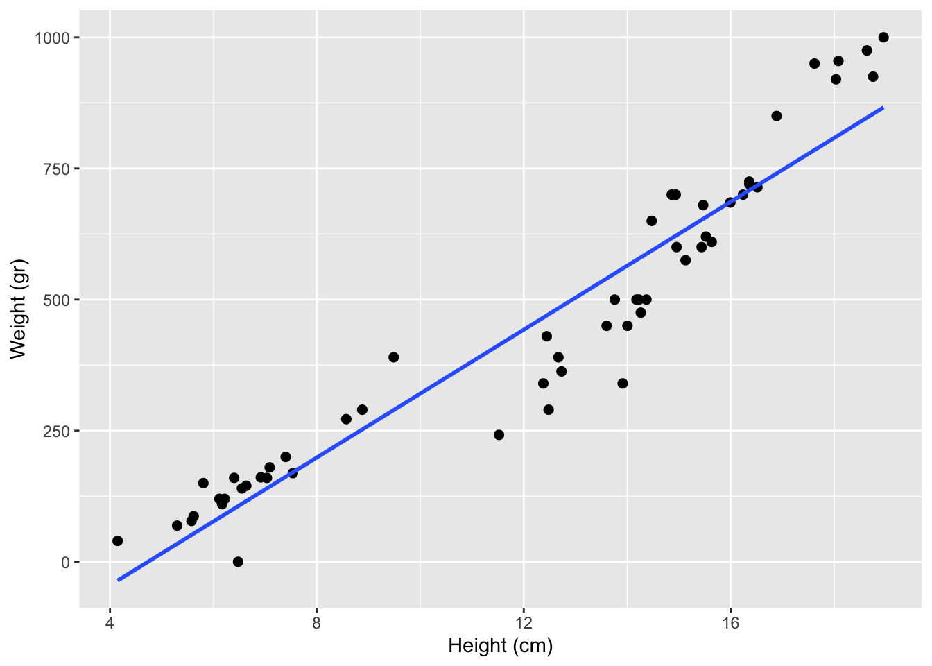
Visualizing the model
Let R draw the line for you!

Visualizing the model
How can we use the line to make predictions?
Predict weight given height:
10 cm
15 cm
20 cm

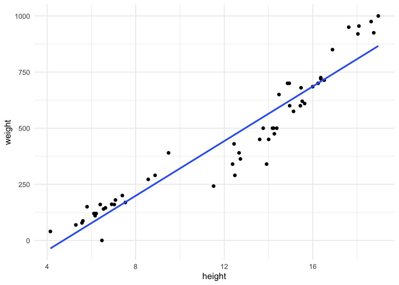
Visualizing the model
Are the predictions good?
Residual: Difference between observed and predicted value
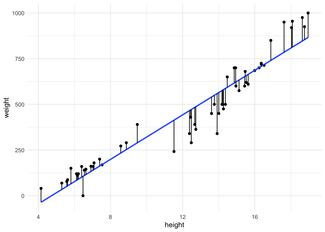
Model evaluation: residuals
Goal: Visualize the residuals
Model evaluation: residuals
Goal: Visualize the residuals
Adding a 3rd Variable
Does the relationship between heights and weights of fish change if we take into consideration species?
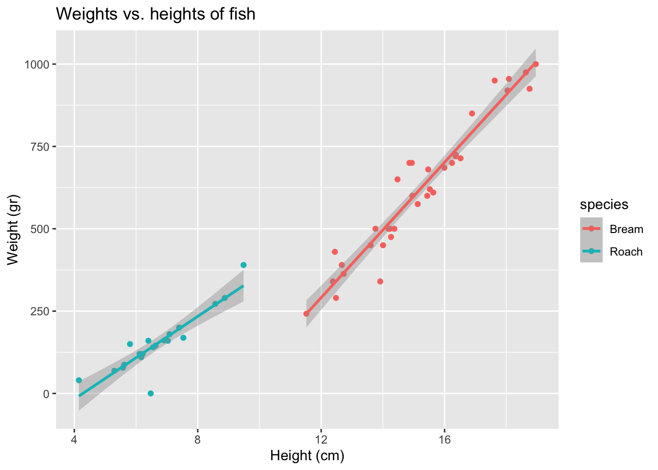
Adding a 3rd Variable
Does the relationship between heights and weights of fish change if we take into consideration species?
