Data Importing

Lecture 9

Midterm Upcoming

• Practice + some review + many more details tomorrow in class

• Initial practice questions are posted!

Lab Check In

Lab 1 Grades

• Please read comments on ALL questions. Some mistakes we did not penalize for, but could in future problems.

• In the first few questions, the point adjustment feature was used for partial credit.

• Regrade requests: submit within a week if you believe a grading mistake was made.

• Code style was the biggest common issue.

  • Even though most questions had code style points, we did not double penalize on this lab.

  • There were some minor problems we did not take off for this time but left comments about.

Code Style

• spaces before and line breaks after each + when building a ggplot,

• spaces before and line breaks after each |> in a data transformation pipeline,

• code should be properly indented

  • this should match the automatic indentation when you hit enter

  • to fix: highlight code, click code option on top of RStudio, select reindent lines

• there should be spaces around = signs and spaces after commas

• use |> and not %>%

• use <- and not = for saving a data frame

Lab 2 clarifications

• Question 7c: No code needed! Use results 7a and 7b to answer. You can delete the code chunk from the template!

• Question 10b: ‘filter your reshaped dataset from question 10’ should be from question 9

• Question 2c: ‘How is the output different from the one in part (a)?’ should say from part (b)

Lab 2 Workflow question

• Select pages on gradescope when you submit

• At least three commits to your lab 2 repo

These should hopefully be free points!!!

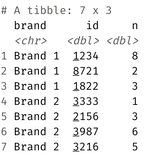
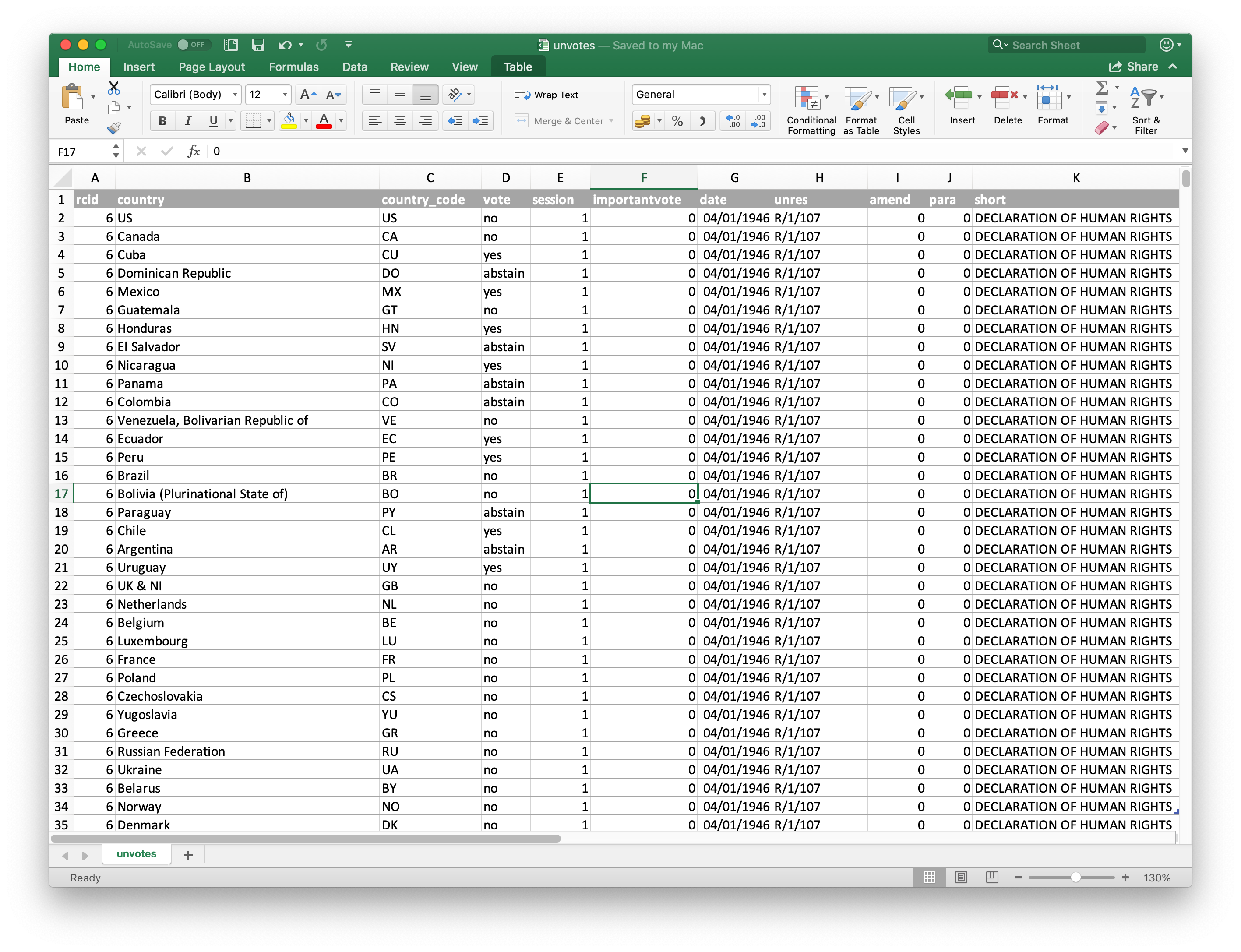
Lab 2 Question 5

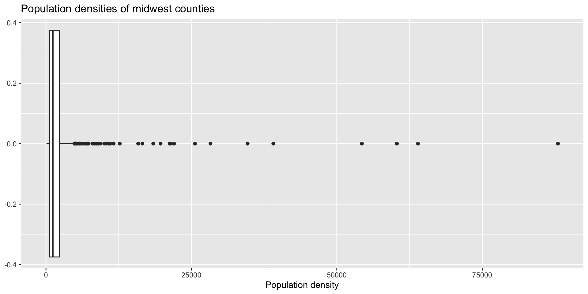
What is a ‘typical value’ of population density?

Lab 2 Question 5

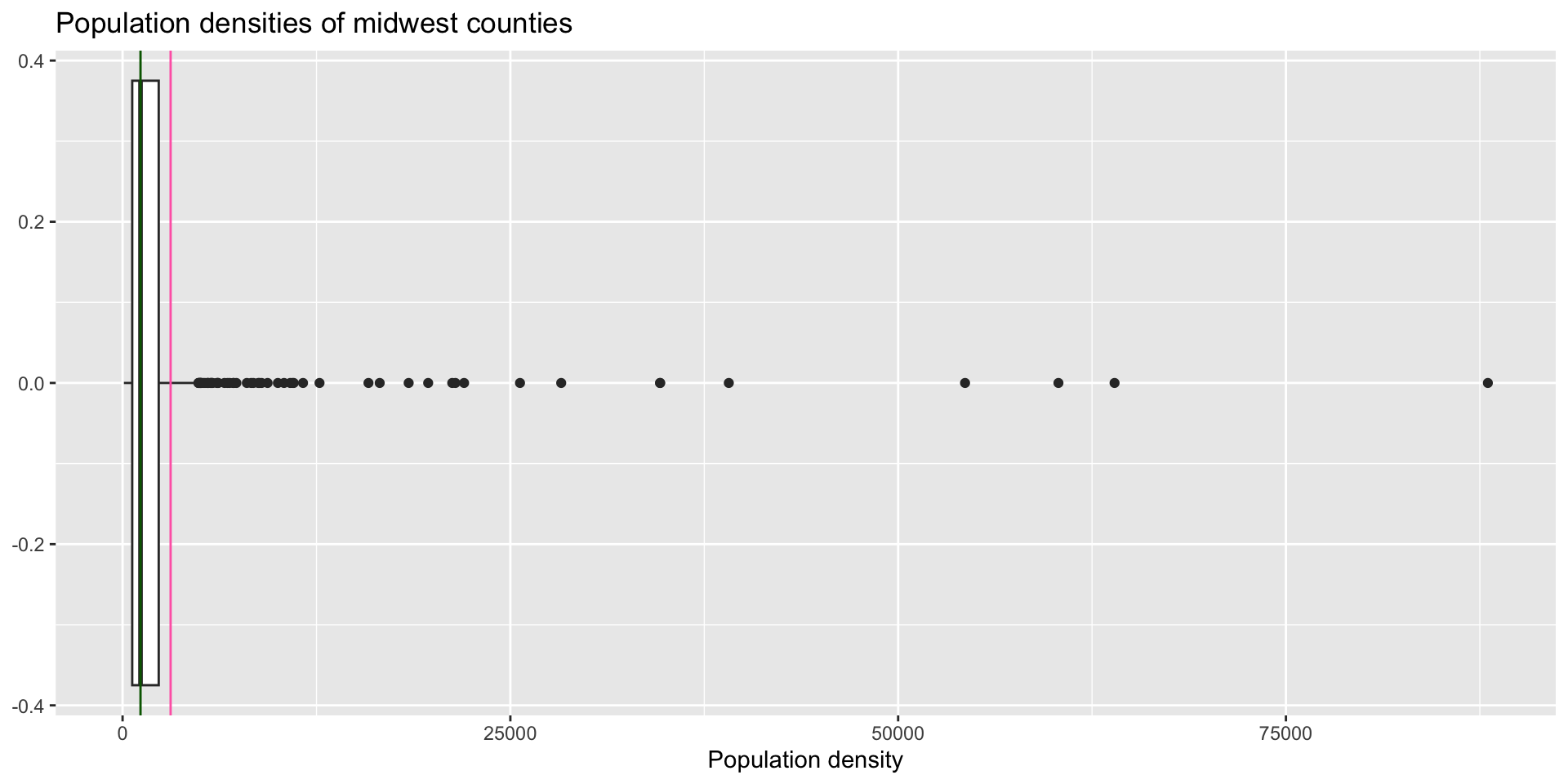
# A tibble: 1 × 2
   mean   med
  <dbl> <dbl>
1 3098. 1156.

Let’s zoom out for a second

Data science and statistical thinking

Before Midterm 1…

• Data science: the real-world art of transforming messy, imperfect, incomplete data into knowledge;

After Midterm 1…

• Statistics: the mathematical discipline of quantifying our uncertainty about that knowledge.

Data science

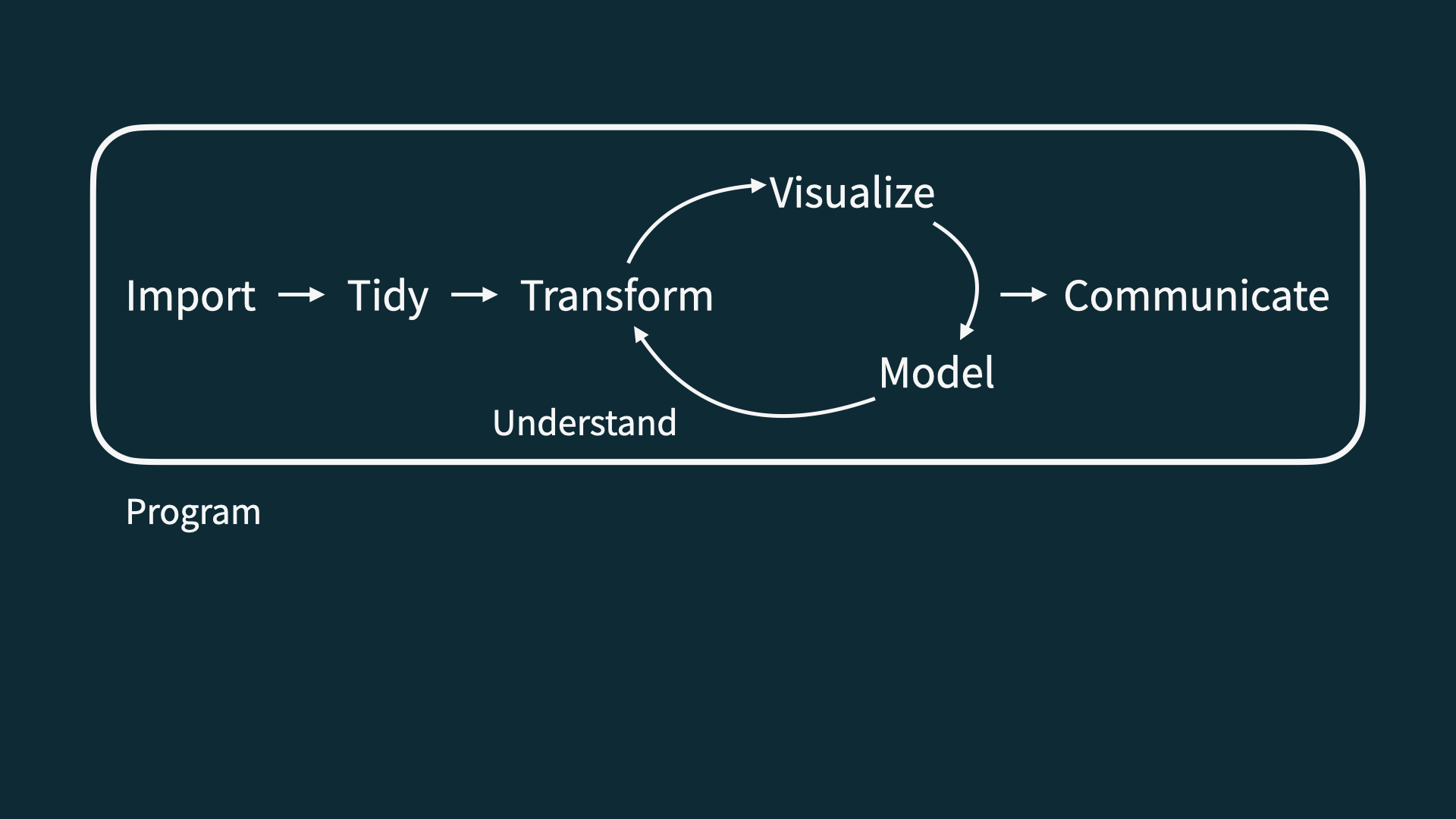
Data science

1. Collection: we won’t seriously study this; data importing coming today

• for us: package data (library()), data importing (read_csv), and webscraping (eventually)
  
• but really: domain-specific issues of measurement, survey design, experimental design, etc
  

Data science

1. Collection: we won’t seriously study this; data importing coming today

2. Preparation: cleaning, wrangling, and otherwise tidying the data so we can actually work with it.

• keywords: mutate, fct_relevel, pivot_*, *_join

Data science

1. Collection: we won’t seriously study this; data importing coming today
2. Preparation: cleaning, wrangling, and otherwise tidying the data so we can actually work with it.

3. Analysis: finally transform the data into knowledge…

• pictures: ggplot, geom_*, etc
  
• numerical summaries: summarize, group_by, count, mean, median, sd, quantile, IQR, cor, etc
  
• The pictures and the summaries need to work together!

Reading data into R

Package data

• When data is in a pack, such as tidyverse, loading the pacakge gets our dataset

• Most often, this is not the case

Reading in rectangular data

Reading rectangular data

• Using readr: (in tidyverse)
  • Most commonly: read_csv() - file saved as .csv
  • Maybe also: read_tsv(), read_delim(), etc - other file formats

. . .

• Using readxl: read_excel() - .xls or .xlsx

. . .

• Using googlesheets4: read_sheet() – We haven’t covered this in the videos, but might be useful for your projects

Using read_csv()

Generally, the format is:

r_df_name <- read_csv("path_to_file_name.csv")

Path to file

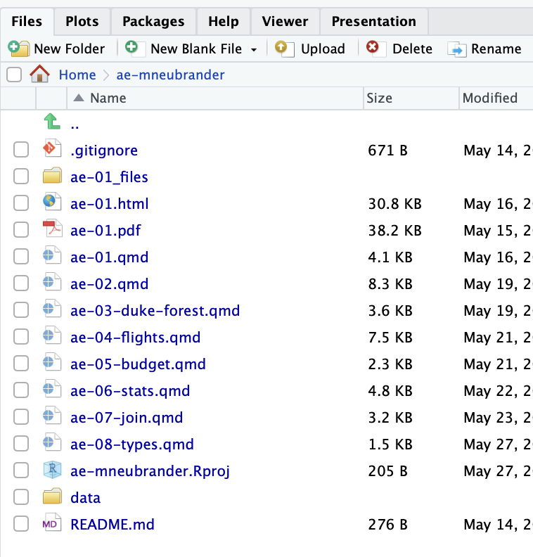
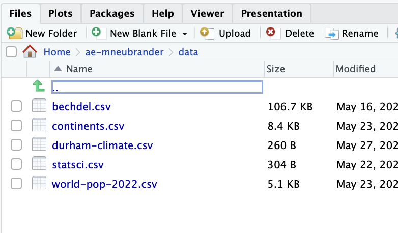
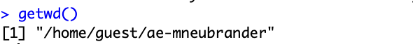
Where is durham-climate.csv?

• use / to separate folder(s) + file names; file path in quotes

• Answer:

Why not include ae-mneubrander?

Where is durham-climate.csv?

We can also write files!

This allows us to save data for later usage, sharing outside of R, etc.

Using write_csv():

write_csv(r_df_name, "path_to_file.csv")

Application exercise

Goal 1.1: Reading and writing CSV files

• Read a CSV file with tidy data

• Split it into subsets based on features of the data

• Write out subsets as CSV files

Goal 1.2: Practice - Case When

• case_when() is similar to if_else(), but allows multiple cases
• case_when() is often used in mutate() to make a new column

df |>
  mutate(new_var = case_when(
    condition_1 ~ result_1,
    condition_2 ~ result_2,
    condition_3 ~ result_3,
    ...,
    .default = default_result
  ))

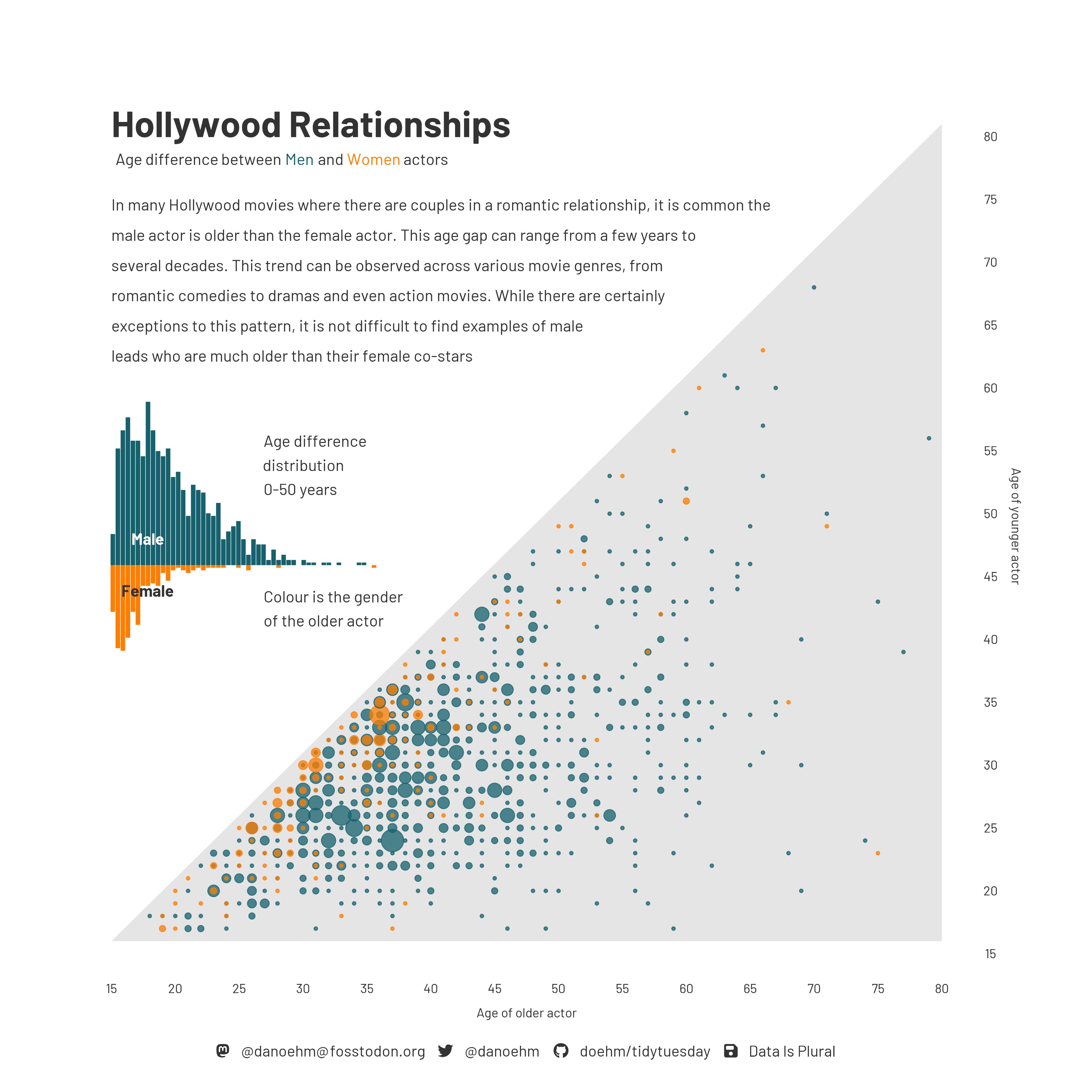
Age gap in Hollywood relationships

Goal 2.1: Reading Excel files & non-tidy data

• Read an Excel file with non-tidy data

• Tidy it up!

Goal 2.2: String Functions

We’ve seen lots of functions that deal with numeric data (mean, median, sum, etc.) - what about characters?

• stringr is a tidyverse package with lots of functions for dealing with character strings

• today: str_detect in stringr

Goal 2.2: String Functions

• str_detect() identifies if some characters are a substring of a larger string

• useful in cases when you need to check some condition, for example:

  • in a filter()

  • in an if_else() or case_when()

Goal 2.2: String Functions

• str_detect() identifies if some characters are a substring of a larger string

• useful in cases when you need to check some condition, for example:

  • in a filter()

  • in an if_else() or case_when()

example: which classes in a list are in the stats department?

classes <- c("sta199", "dance122", "math185", "sta240", "pubpol202")
str_detect(classes, "sta")

[1]  TRUE FALSE FALSE  TRUE FALSE

Goal 2.2: String Functions

General form:

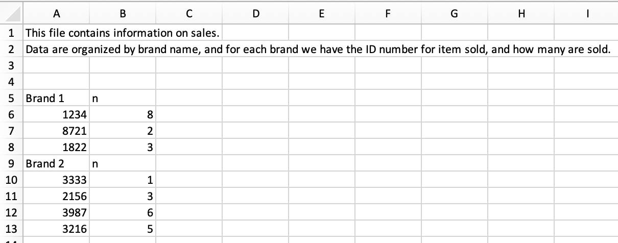
str_detect(character_var, "word_to_detect")

Sales data

. . .

Are these data tidy? Why or why not?

Sales data

What “data moves” do we need to go from the original, non-tidy data to this, tidy one?