Announcement: Office Hours/Exam
Teaching Evaluation
Teaching evaluations due tomorrow. If we get 13/17 responses, I’ll add +2 points to everyone’s final exam grade!
Current Grade Calculation
-
AEs: 5%: completion of 80% or more is full credits
Lab Attendance: 5% - one drop given (score - number of labs out of 10)
Labs: 30% - Lowest is dropped (5 labs at 6% each)
Midterm - 20% (Add in-class + take-home score to get total out of 100)
Project - 20%
Final - 20%
. . .
If you do better on the final than the midterm, it will be weighted higher!
Final Overview
- All multiple choice (same format as midterm in-class)
- Cumulative!!!
- Cheat sheet: 2 pages front and back
Content Review
What model should I use?
First, look at what type of output you have:
Numerical: Linear regression
Binary: Logistic regression
Other: We haven’t learned how to do this!
What model should I use?
Now, look at your predictors. Does the relationship between the output and each predictor stay the same regardless of other predictors?
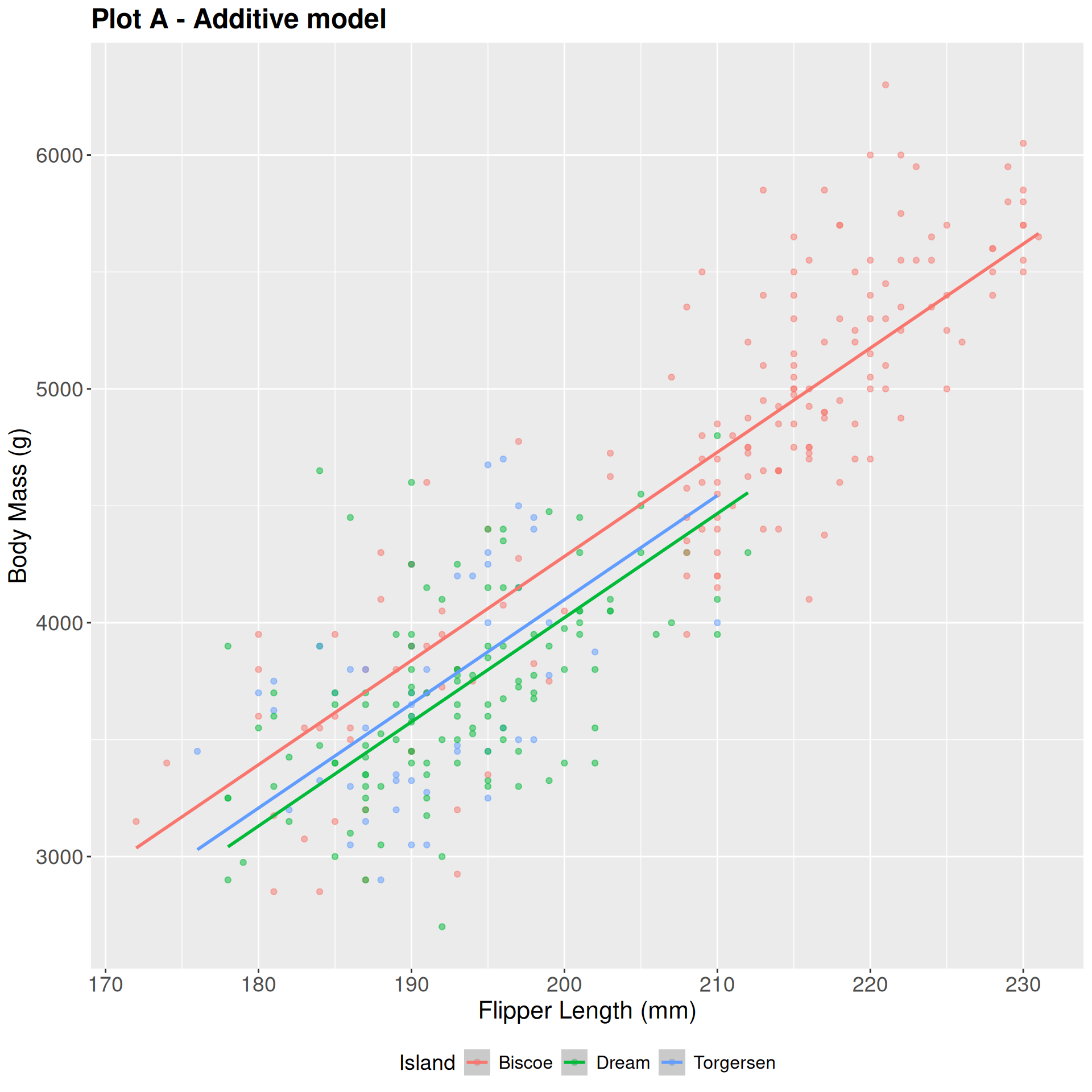
Yes: Additive
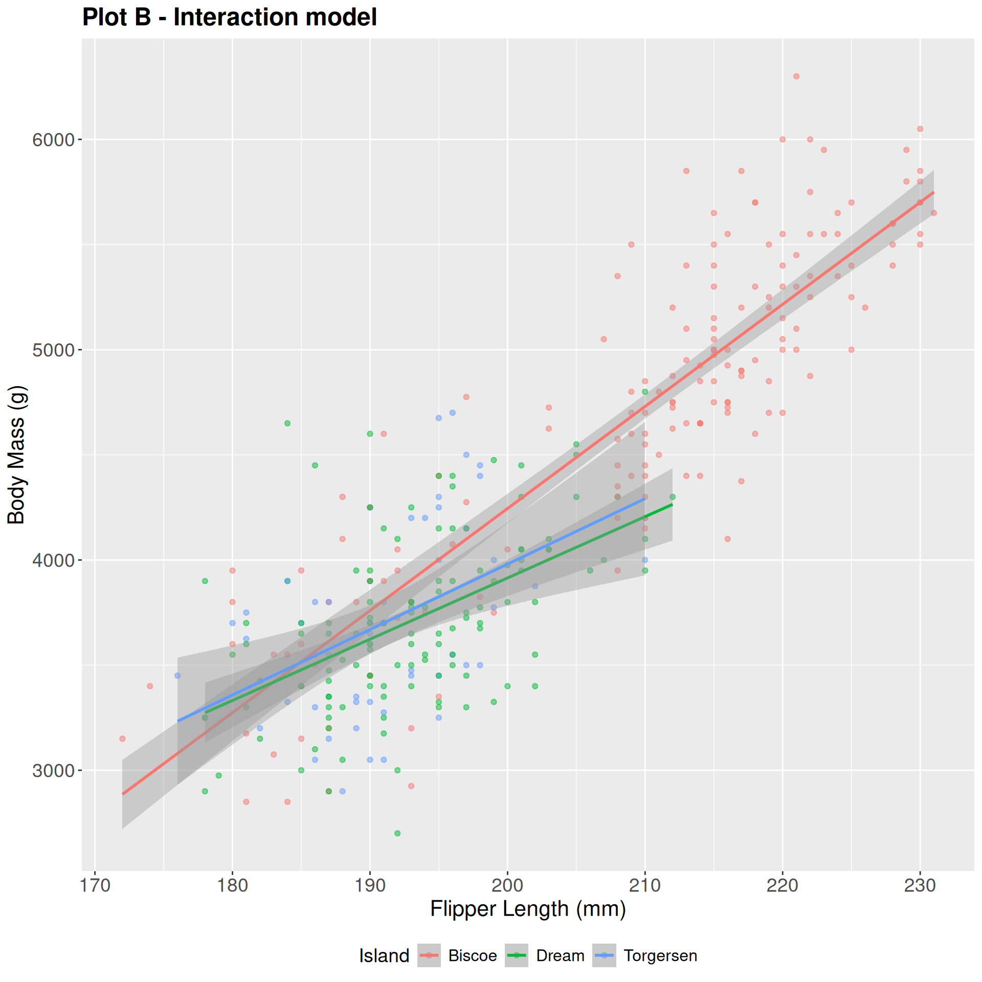
No: interaction
Practice
# A tibble: 6 × 3
  did_rain temperature humidity
  <fct>          <dbl>    <dbl>
1 no_rain         71.4     52.7
2 rain            66.3     80
3 no_rain         70.3     53.1
4 rain            63.3     88.8
5 rain            60.2     77.5
6 no_rain         76.7     65.9
- What type of model to predict
did_rain from temperature?
- What type of model to predict
temperature from did_rain?
- What type of model to predict
humidity from did_rain and and temperature?
- What type of model to predict
did_rain from temperature and humidity?
Model comparison
-
Linear Regression:
-
Logistic Regression:
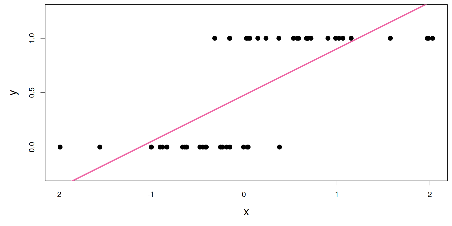
Review: Logistic Regression
Line of best fit? A little silly…
What is the s-curve??
It’s the logistic function:
\[
\text{Prob}(y = 1)
=
\frac{e^{\beta_0+\beta_1x}}{1+e^{\beta_0+\beta_1x}}.
\]
. . .
If you set \(p = \text{Prob}(y = 1)\) and do some algebra, you get the simple linear model for the log-odds:
. . .
\[
\log\left(\frac{p}{1-p}\right)
=
\beta_0+\beta_1x.
\]
. . .
This is called the logistic regression model.
Estimation
. . .
\[
\log\left(\frac{\widehat{p}}{1-\widehat{p}}\right)
=
b_0+b_1x.
\]
. . .
-
\(\hat{p}\) is the predicted probability that \(y = 1\)
- In R, the second level of the factor is taken as \(y = 1\)
Interpreting the intercept
Plug in \(x = 0\):
\[
\log\left(\frac{\widehat{p}}{1-\widehat{p}}\right)
=
b_0+b_1x.
\]
. . .
When \(x = 0\), the estimated log-odds is \(b_0\).
. . .
When \(x = 0\), the estimated probability that \(y = 1\) is
\[
\hat{p} = \frac{e^{b_0}}{1+e^{b_0}}
\]
Interpreting the slope is tricky
Recall:
\[
\log\left(\frac{\widehat{p}}{1-\widehat{p}}\right)
=
b_0+b_1x.
\]
. . .
Alternatively:
\[
\frac{\widehat{p}}{1-\widehat{p}}
=
e^{b_0+b_1x}
=
\color{blue}{e^{b_0}e^{b_1x}}
.
\]
. . .
If we increase \(x\) by one unit, we have:
\[
\frac{\widehat{p}}{1-\widehat{p}}
=
e^{b_0}e^{b_1(x+1)}
=
e^{b_0}e^{b_1x+b_1}
=
{\color{blue}{e^{b_0}e^{b_1x}}}{\color{red}{e^{b_1}}}
.
\]
. . .
A one unit increase in \(x\) is associated with a change in odds by a factor of \(e^{b_1}\). Gross!
Sign of the slope is meaningful
A one unit increase in \(x\) is associated with a change in odds by a factor of \(e^{b_1}\).
. . .
- A positive slope means increasing \(x\) increases the odds (and probability!) that \(y = 1\)
- A negative slope means increasing \(x\) decreases the odds (and probability!) that \(y = 1\)
Threshold
Pick some probability threshold \(p^*\).
- If \(\hat{p} > p^*\) - predict \(y = 1\)
- If \(\hat{p} < p^*\) - predict \(y = 0\)
. . .
The higher the threshold, the harder it is to classify as \(y = 1\)!!!
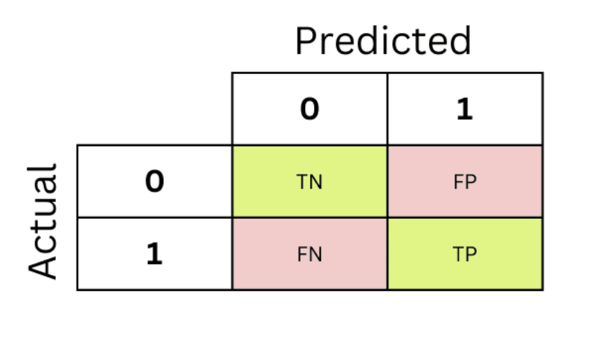
Classification Rates
- False negative rate = \(\frac{FN}{FN + TP}\)
- False positive rate = \(\frac{FP}{FP + TN}\)
- Sensitivity = \(\frac{FN}{FN + TP}\) = 1 − False negative rate
- Specificity = \(\frac{TN}{FP + TN}\) = 1 - False positive rate
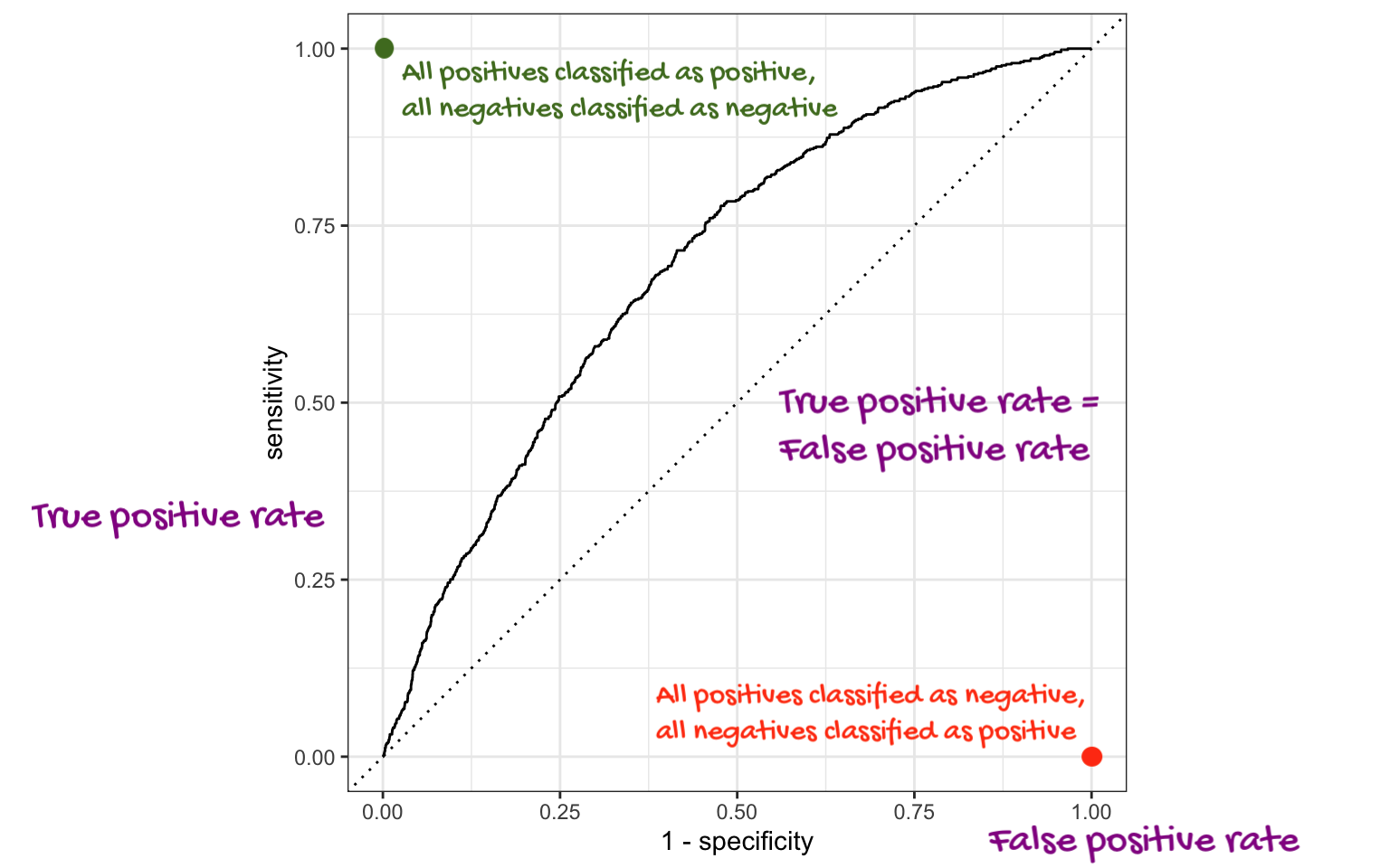
ROC Curve + AUC
. . .
AUC: Area under the curve
“Three branches of statistical government”
We have an unknown quantity we are trying to learn about (for example, \(\beta_1\)) using noisy, imperfect data. Learning comes in three flavors:
POINT ESTIMATION: get a single-number best guess for \(\beta_1\);
INTERVAL ESTIMATION: get a range of likely values for \(\beta_1\) that characterizes (sampling) uncertainty;
HYPOTHESIS TESTING: use the data to distinguish competing claims about \(\beta_1\).