More logistic regression

Lecture 19

Published

June 19, 2025

While you wait…

  • Go to your ae project in RStudio.

  • Make sure all of your changes up to this point are committed and pushed, i.e., there’s nothing left in your Git pane.

  • Click Pull to get today’s application exercise file: ae-14-spam-filter.qmd.

  • Wait till the you’re prompted to work on the application exercise during class before editing the file.

Announcements

  • Office hours tomorrow will be about 20 mins short (1:00 - 2:40). I will be there a little before 1:00 if you want to come early!

  • Make appointment to see in-class exams/talk through problems you’re stuck on. Remember, final exam is cumulative!!

Project Reminders

  • Milestone 3 due Friday night!!

  • Once your project website renders, you still need to push for the changes to show up!!!

Logistic Regression: Recap

Goal: modelling/predicting binary outcome \(y\)

  • Idea: Model the probability \(p\) that \(y = 1\)

. . .

  • S-curve for the probability of success \(p=P(y=1)\):

\[ \hat{p} = \frac{e^{b_0+b_1x}}{1+e^{b_0+b_1x}}. \]

. . .

  • Linear model for the log-odds:

\[ \log\left(\frac{\hat{p}}{1-\hat{p}}\right) = b_0+b_1x. \]

R syntax is mostly unchanged

simple_logistic_fit <- logistic_reg() |>
  fit(spam ~ exclaim_mess, data = email)

tidy(simple_logistic_fit)
# A tibble: 2 × 5
  term          estimate std.error statistic p.value
  <chr>            <dbl>     <dbl>     <dbl>   <dbl>
1 (Intercept)  -2.27      0.0553     -41.1     0    
2 exclaim_mess  0.000272  0.000949     0.287   0.774

. . .

Fitted equation for the log-odds:

\[ \log\left(\frac{\hat{p}}{1-\hat{p}}\right) = -2.27 + 0.000272\times exclaim~mess \]

. . .

Interpretations are strange and delicate.

Questions??? Review??? Anything?!

Let’s Practice

AE-14: Watch now, fill in later (optional!)

Goal

  • We will build a spam filter from email data
  • The data come from incoming emails in David Diez’s (one of the authors of OpenIntro textbooks) Gmail account for the first three months of 2012
  • User number of exclamation marks in an email address (exclaim_mess) to predict whether or not the email is spam (spam: 1 if spam; 0 if not)

Data

glimpse(email)
Rows: 3,921
Columns: 21
$ spam         <fct> 0, 0, 0, 0, 0, 0, 0, 0, 0, 0, 0, 0, 0, 0, 0, 0,…
$ to_multiple  <fct> 0, 0, 0, 0, 0, 0, 1, 1, 0, 0, 0, 0, 0, 0, 0, 0,…
$ from         <fct> 1, 1, 1, 1, 1, 1, 1, 1, 1, 1, 1, 1, 1, 1, 1, 1,…
$ cc           <int> 0, 0, 0, 0, 0, 0, 0, 1, 0, 0, 0, 1, 0, 1, 2, 1,…
$ sent_email   <fct> 0, 0, 0, 0, 0, 0, 1, 1, 0, 0, 1, 0, 0, 1, 0, 1,…
$ time         <dttm> 2012-01-01 06:16:41, 2012-01-01 07:03:59, 2012…
$ image        <dbl> 0, 0, 0, 0, 0, 0, 0, 1, 0, 0, 0, 0, 0, 0, 0, 0,…
$ attach       <dbl> 0, 0, 0, 0, 0, 0, 0, 1, 0, 0, 0, 0, 0, 0, 0, 0,…
$ dollar       <dbl> 0, 0, 4, 0, 0, 0, 0, 0, 0, 0, 0, 0, 0, 0, 2, 0,…
$ winner       <fct> no, no, no, no, no, no, no, no, no, no, no, no,…
$ inherit      <dbl> 0, 0, 1, 0, 0, 0, 0, 0, 0, 0, 0, 0, 0, 0, 0, 0,…
$ viagra       <dbl> 0, 0, 0, 0, 0, 0, 0, 0, 0, 0, 0, 0, 0, 0, 0, 0,…
$ password     <dbl> 0, 0, 0, 0, 2, 2, 0, 0, 0, 0, 0, 0, 0, 0, 0, 0,…
$ num_char     <dbl> 11.370, 10.504, 7.773, 13.256, 1.231, 1.091, 4.…
$ line_breaks  <int> 202, 202, 192, 255, 29, 25, 193, 237, 69, 68, 2…
$ format       <fct> 1, 1, 1, 1, 0, 0, 1, 1, 0, 1, 1, 0, 1, 1, 1, 1,…
$ re_subj      <fct> 0, 0, 0, 0, 0, 0, 0, 0, 0, 0, 0, 1, 0, 1, 1, 1,…
$ exclaim_subj <dbl> 0, 0, 0, 0, 0, 0, 0, 0, 0, 0, 0, 0, 0, 0, 0, 0,…
$ urgent_subj  <fct> 0, 0, 0, 0, 0, 0, 0, 0, 0, 0, 0, 0, 0, 0, 0, 0,…
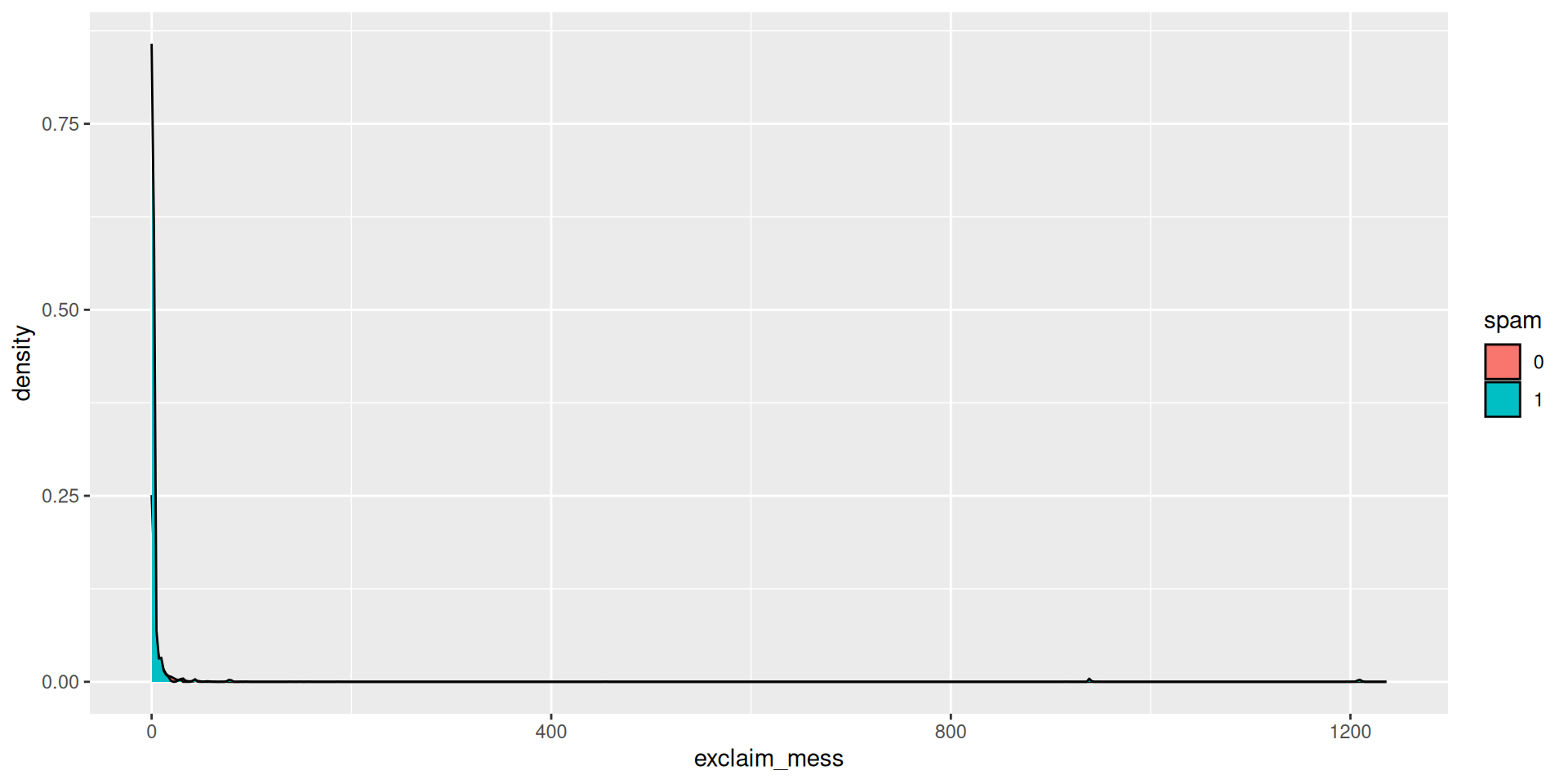
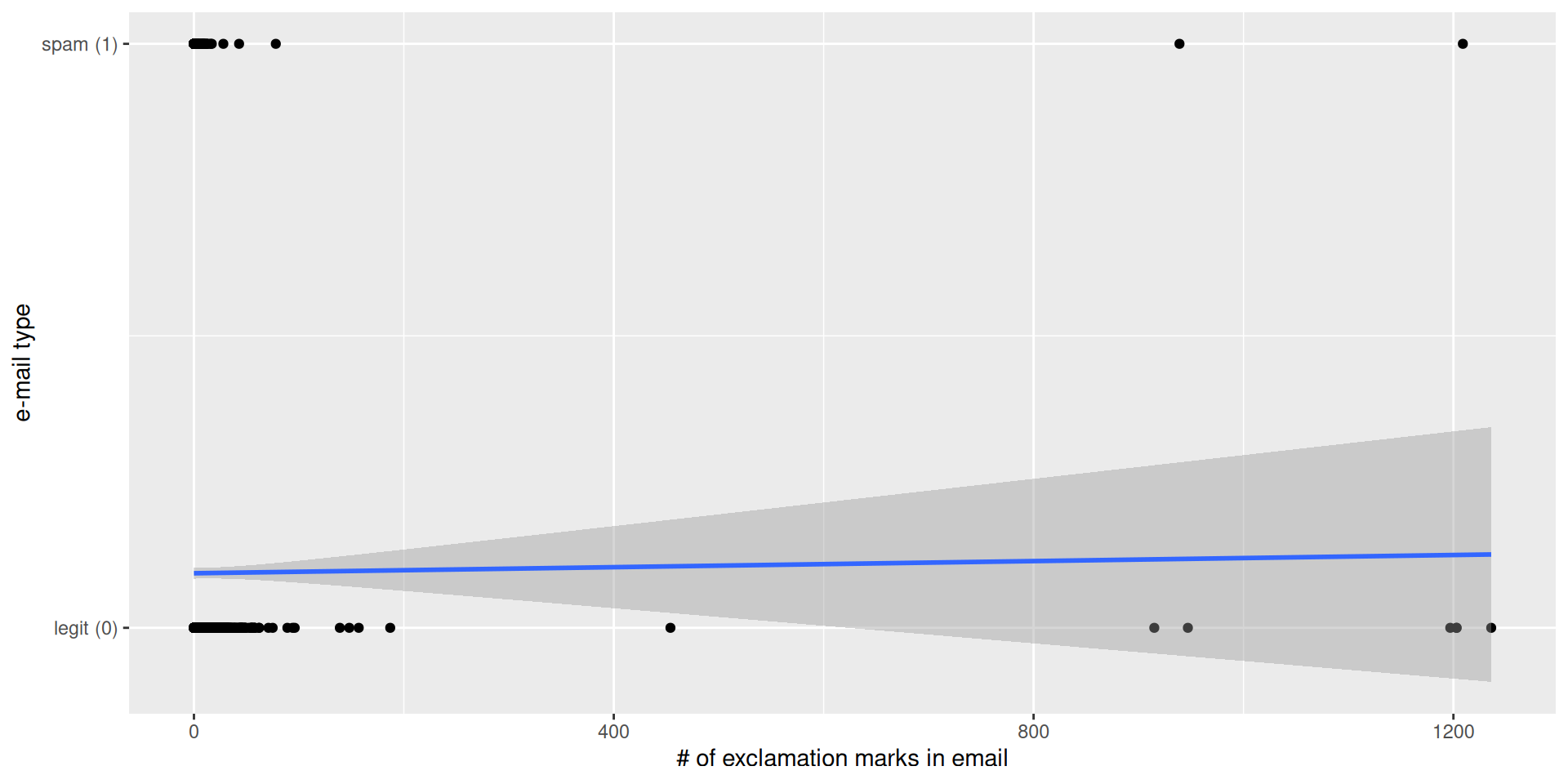
$ exclaim_mess <dbl> 0, 1, 6, 48, 1, 1, 1, 18, 1, 0, 2, 1, 0, 10, 4,…
$ number       <fct> big, small, small, small, none, none, big, smal…

EDA (Ex. 1)

EDA (Ex. 1)

Mean exclamation points by spam/not spam:

# A tibble: 2 × 2
  spam  mean_ep
  <fct>   <dbl>
1 0        6.51
2 1        7.32

Linear Model (Ex. 2)

This makes no sense at all.

Fit Logistic Regression (Ex. 3)

This is what we have seen already!

spam_exl_fit <- logistic_reg() |>
  fit(spam ~ exclaim_mess, data = email)

tidy(spam_exl_fit)
# A tibble: 2 × 5
  term          estimate std.error statistic p.value
  <chr>            <dbl>     <dbl>     <dbl>   <dbl>
1 (Intercept)  -2.27      0.0553     -41.1     0    
2 exclaim_mess  0.000272  0.000949     0.287   0.774

\[ \log\left(\frac{\hat{p}}{1-\hat{p}}\right) = -2.27 + 0.000272\times exclaim~mess \]

Goal: Predict!! (Ex. 4a)

What is the probability the email is spam if it contains 10 exclamation points?? Use predict!

new_email <- tibble(
  exclaim_mess = 10
  )

new_email
# A tibble: 1 × 1
  exclaim_mess
         <dbl>
1           10

Goal: Predict!! (Ex. 4a)

What is the probability the email is spam if it contains 10 exclamation points?? Use predict!

new_email <- tibble(
  exclaim_mess = 10
  )

predict(spam_exl_fit, new_data = new_email, type = "prob")
# A tibble: 1 × 2
  .pred_0 .pred_1
    <dbl>   <dbl>
1   0.906  0.0937

Goal: Predict!! (Ex. 4b)

A probability is nice, but we want an actual decision. Classify the email!!!

predict(spam_exl_fit, new_data = new_email, type = "class")
# A tibble: 1 × 1
  .pred_class
  <fct>      
1 0          

. . .

The default behavior is to threshold the probabilities by 0.5.

Let’s use more data (Ex. 5a)

Why limit ourselves to using exclamation points???

spam_fit <- logistic_reg() |>
  fit(spam ~ time + exclaim_mess + line_breaks, data = email)

Let’s use even more data (Ex. 5b)

What about all the predictors???

spam_all_fit <- logistic_reg() |>
  fit(spam ~ ., data = email)
Warning: glm.fit: fitted probabilities numerically 0 or 1 occurred

The . means all other variables .

Is our model good??? (Ex. 5c)

  • Goal is to evaluate how good our model is.
  • If you’re coding along: pause!! We’re going to review concepts first!!

Reminder: Classification Error

There are two kinds of mistakes:

We want to avoid both, but there’s a trade-off.

Terms: False negative and positive rates

  • False negative rate is the proportion of actual positives that were classified as negatives.

  • False positive rate is the proportion of actual negatives that were classified as positives.

. . .

Tip

We want these to be low!

Terms: False negative and positive rates

  • False negative rate = \(\frac{FN}{FN + TP}\)

  • False positive rate = \(\frac{FP}{FP + TN}\)

Term: Sensitivity

Sensitivity is the proportion of actual positives that were correctly classified as positive.

  • Also known as true positive rate and recall

  • Sensitivity = \(\frac{FN}{FN + TP}\)

  • Sensitivity = 1 − False negative rate

  • Useful when false negatives are more “expensive” than false positives

Tip

We want this to be high!

Term: Specificity

Specificity is the proportion of actual negatives that were correctly classified as negative

  • Also known as true negative rate

  • Specificity = \(\frac{TN}{FP + TN}\)

  • Specificity = 1 − False positive rate

  • Useful when false positives are more “expensive” than false negatives

Tip

We want this to be high!

The augment function

The augment function takes a data frame and “augments” it by adding three new columns on the left that describe the model predictions for each row:

  • .pred_class: model prediction (\(\hat{y}\)) based on a 50% threshold;
  • .pred_0: model estimate of \(P(y=0)\);
  • .pred_1: model estimate of \(P(y=1) = 1 - P(y = 0)\).

The augment function

The augment function takes a data frame and “augments” it by adding three new columns on the left that describe the model predictions for each row:

spam_aug_all <- augment(spam_all_fit, email)
spam_aug_all
# A tibble: 3,921 × 24
   .pred_class .pred_0  .pred_1 spam  to_multiple from     cc
   <fct>         <dbl>    <dbl> <fct> <fct>       <fct> <int>
 1 0             0.867 1.33e- 1 0     0           1         0
 2 0             0.943 5.70e- 2 0     0           1         0
 3 0             0.942 5.78e- 2 0     0           1         0
 4 0             0.920 7.96e- 2 0     0           1         0
 5 0             0.903 9.74e- 2 0     0           1         0
 6 0             0.901 9.87e- 2 0     0           1         0
 7 0             1.00  7.89e-12 0     1           1         0
 8 0             1.00  1.24e-12 0     1           1         1
 9 0             0.862 1.38e- 1 0     0           1         0
10 0             0.922 7.76e- 2 0     0           1         0
# ℹ 3,911 more rows
# ℹ 17 more variables: sent_email <fct>, time <dttm>, image <dbl>,
#   attach <dbl>, dollar <dbl>, winner <fct>, inherit <dbl>,
#   viagra <dbl>, password <dbl>, num_char <dbl>, line_breaks <int>,
#   format <fct>, re_subj <fct>, exclaim_subj <dbl>,
#   urgent_subj <fct>, exclaim_mess <dbl>, number <fct>

Calculating the error rates (5c)

spam_aug_all |>
  count(spam, .pred_class) 
# A tibble: 4 × 3
  spam  .pred_class     n
  <fct> <fct>       <int>
1 0     0            3521
2 0     1              33
3 1     0             299
4 1     1              68

Calculating the error rates (5c)

spam_aug_all |>
  count(spam, .pred_class) |>
  group_by(spam)
# A tibble: 4 × 3
# Groups:   spam [2]
  spam  .pred_class     n
  <fct> <fct>       <int>
1 0     0            3521
2 0     1              33
3 1     0             299
4 1     1              68

Calculating the error rates (5c)

spam_aug_all |>
  count(spam, .pred_class) |>
  group_by(spam) |>
  mutate(p = n / sum(n))
# A tibble: 4 × 4
# Groups:   spam [2]
  spam  .pred_class     n       p
  <fct> <fct>       <int>   <dbl>
1 0     0            3521 0.991  
2 0     1              33 0.00929
3 1     0             299 0.815  
4 1     1              68 0.185  

Calculating the error rates (5c)

spam_aug_all |>
  count(spam, .pred_class) |>
  group_by(spam) |>
  mutate(p = n / sum(n),
         decision = case_when(
            spam == "0" & .pred_class == "0" ~ "True negative",
            spam == "0" & .pred_class == "1" ~ "False positive",
            spam == "1" & .pred_class == "0" ~ "False negative",
            spam == "1" & .pred_class == "1" ~ "True positive"
        ))
# A tibble: 4 × 5
# Groups:   spam [2]
  spam  .pred_class     n       p decision      
  <fct> <fct>       <int>   <dbl> <chr>         
1 0     0            3521 0.991   True negative 
2 0     1              33 0.00929 False positive
3 1     0             299 0.815   False negative
4 1     1              68 0.185   True positive 

This is where we have AE14 stop….

But wait!

Augment uses a default 50% threshold.

. . .

If we change the classification threshold, we change the classifications, and we change the error rates:

. . .

spam_aug_all |>
  mutate(
    .pred_class = if_else(.pred_1 <= 0.25, 0, 1)
  ) |>
  count(spam, .pred_class) |>
  group_by(spam) |>
  mutate(p = n / sum(n))
# A tibble: 4 × 4
# Groups:   spam [2]
  spam  .pred_class     n      p
  <fct>       <dbl> <int>  <dbl>
1 0               0  3263 0.918 
2 0               1   291 0.0819
3 1               0   172 0.469 
4 1               1   195 0.531 

Classification threshold: 0.00

spam_aug_all |>
  mutate(
    .pred_class = if_else(.pred_1 <= 0.00, 0, 1)
  ) |>
  count(spam, .pred_class) |>
  group_by(spam) |>
  mutate(p = n / sum(n))
# A tibble: 2 × 4
# Groups:   spam [2]
  spam  .pred_class     n     p
  <fct>       <dbl> <int> <dbl>
1 0               1  3554     1
2 1               1   367     1

Classification threshold: 0.25

spam_aug_all |>
  mutate(
    .pred_class = if_else(.pred_1 <= 0.25, 0, 1)
  ) |>
  count(spam, .pred_class) |>
  group_by(spam) |>
  mutate(p = n / sum(n))
# A tibble: 4 × 4
# Groups:   spam [2]
  spam  .pred_class     n      p
  <fct>       <dbl> <int>  <dbl>
1 0               0  3263 0.918 
2 0               1   291 0.0819
3 1               0   172 0.469 
4 1               1   195 0.531 

Classification threshold: 0.5

spam_aug_all |>
  mutate(
    .pred_class = if_else(.pred_1 <= 0.50, 0, 1)
  ) |>
  count(spam, .pred_class) |>
  group_by(spam) |>
  mutate(p = n / sum(n))
# A tibble: 4 × 4
# Groups:   spam [2]
  spam  .pred_class     n       p
  <fct>       <dbl> <int>   <dbl>
1 0               0  3521 0.991  
2 0               1    33 0.00929
3 1               0   299 0.815  
4 1               1    68 0.185  

Classification threshold: 0.75

spam_aug_all |>
  mutate(
    .pred_class = if_else(.pred_1 <= 0.75, 0, 1)
  ) |>
  count(spam, .pred_class) |>
  group_by(spam) |>
  mutate(p = n / sum(n))
# A tibble: 4 × 4
# Groups:   spam [2]
  spam  .pred_class     n       p
  <fct>       <dbl> <int>   <dbl>
1 0               0  3544 0.997  
2 0               1    10 0.00281
3 1               0   339 0.924  
4 1               1    28 0.0763 

Classification threshold: 1.00

spam_aug_all |>
  mutate(
    .pred_class = if_else(.pred_1 <= 1.00, 0, 1)
  ) |>
  count(spam, .pred_class) |>
  group_by(spam) |>
  mutate(p = n / sum(n))
# A tibble: 2 × 4
# Groups:   spam [2]
  spam  .pred_class     n     p
  <fct>       <dbl> <int> <dbl>
1 0               0  3554     1
2 1               0   367     1

Let’s plot these error rates

ROC curve

If we repeat this process for “all” possible thresholds \(0\leq p^\star\leq 1\), we trace out the receiver operating characteristic curve (ROC curve), which assesses the model’s performance across a range of thresholds:

ROC curve

Which corner of the plot indicates the best model performance?

. . .

Upper left!

Model comparison

The farther up and to the left the ROC curve is, the better the classification accuracy. You can quantify this with the area under the curve.

Note

Area under the ROC curve will be our “quality score” for comparing logistic regression models.

ROC for full model

ROC for simple model

Should we include a predictor?

To determine whether we should include a predictor in a model, we should start by asking:

  • Is it ethical to use this variable? (Or even legal?)

  • Will this variable be available at prediction time?

  • Does this variable contribute to explainability?

Data splitting and spending

We’ve been cheating!

  • So far, we’ve been using all the data we have for building models. In predictive contexts, this would be considered cheating.

  • Evaluating model performance for predicting outcomes that were used when building the models is like evaluating your learning with questions whose answers you’ve already seen.

Spending your data

For predictive models (used primarily in machine learning), we typically split data into training and test sets:

- The training set is used for EDA (plots, summary statistics, etc.)

  • The training set is used to estimate model parameters (fit models).

  • The test set is used to find an independent assessment of model performance. NEVER look at the test set during training.

How much to spend?

  • The more data we spend (use in training), the better estimates we’ll get.

  • Spending too much data in training prevents us from computing a good assessment of predictive performance.

  • Spending too much data in testing prevents us from computing a good estimate of model parameters.

The initial split

Randomly pick training and testing rows!

set.seed(20241112)
email_split <- initial_split(email)
email_split
<Training/Testing/Total>
<2940/981/3921>

. . .

Default: 75% training; 25% testing

The initial split

Change proportion:

set.seed(20250612)
email_split <- initial_split(email, prop = 0.8)
email_split
<Training/Testing/Total>
<3136/785/3921>

Setting a seed

What does set.seed() do?

  • To create that split of the data, R generates “pseudo-random” numbers: while they are made to behave like random numbers, their generation is deterministic given a “seed”.

  • This allows us to reproduce results by setting that seed.

  • Which seed you pick doesn’t matter, as long as you don’t try a bunch of seeds and pick the one that gives you the best performance.

Accessing the data

email_train <- training(email_split)
email_test <- testing(email_split)

The training set

email_train
# A tibble: 3,136 × 21
   spam  to_multiple from     cc sent_email time                image
   <fct> <fct>       <fct> <int> <fct>      <dttm>              <dbl>
 1 0     0           1         0 0          2012-02-18 19:20:54     0
 2 1     0           1         0 0          2012-03-10 22:43:58     0
 3 0     1           1         0 0          2012-03-06 14:10:00     0
 4 1     0           1         0 0          2012-03-18 13:26:41     0
 5 0     0           1         0 1          2012-03-16 00:47:33     0
 6 0     0           1         0 1          2012-03-31 13:24:03     0
 7 0     0           1         0 0          2012-02-16 16:25:22     0
 8 0     0           1         0 0          2012-02-24 23:18:35     0
 9 0     1           1         0 1          2012-01-22 09:02:27     0
10 0     0           1         0 0          2012-02-11 00:46:30     0
# ℹ 3,126 more rows
# ℹ 14 more variables: attach <dbl>, dollar <dbl>, winner <fct>,
#   inherit <dbl>, viagra <dbl>, password <dbl>, num_char <dbl>,
#   line_breaks <int>, format <fct>, re_subj <fct>,
#   exclaim_subj <dbl>, urgent_subj <fct>, exclaim_mess <dbl>,
#   number <fct>

The testing data

email_test
# A tibble: 785 × 21
   spam  to_multiple from     cc sent_email time                image
   <fct> <fct>       <fct> <int> <fct>      <dttm>              <dbl>
 1 0     1           1         1 1          2012-01-01 18:45:21     1
 2 0     0           1         0 1          2012-01-01 18:23:44     0
 3 0     0           1         1 1          2012-01-01 23:40:14     0
 4 0     0           1         0 0          2012-01-02 02:51:24     0
 5 0     0           1         2 0          2012-01-02 04:07:57     0
 6 0     0           1         0 0          2012-01-02 14:35:56     0
 7 0     0           1         0 0          2012-01-02 15:12:51     0
 8 0     0           1         5 0          2012-01-02 17:48:26     0
 9 0     1           1         1 0          2012-01-02 15:27:07     0
10 0     0           1         7 0          2012-01-03 00:07:51     0
# ℹ 775 more rows
# ℹ 14 more variables: attach <dbl>, dollar <dbl>, winner <fct>,
#   inherit <dbl>, viagra <dbl>, password <dbl>, num_char <dbl>,
#   line_breaks <int>, format <fct>, re_subj <fct>,
#   exclaim_subj <dbl>, urgent_subj <fct>, exclaim_mess <dbl>,
#   number <fct>

AE 15

  • Create a train and test split
  • Fit models
  • Test and evaluate models

Washington forests

Data

  • The U.S. Forest Service maintains machine learning models to predict whether a plot of land is “forested.”

  • This classification is important for research, legislation, land management, etc. purposes.

  • Plots are typically remeasured every 10 years.

  • The forested dataset contains the most recent measurement per plot.

Data: forested

forested
# A tibble: 7,107 × 19
   forested  year elevation eastness northness roughness tree_no_tree
   <fct>    <dbl>     <dbl>    <dbl>     <dbl>     <dbl> <fct>       
 1 Yes       2005       881       90        43        63 Tree        
 2 Yes       2005       113      -25        96        30 Tree        
 3 No        2005       164      -84        53        13 Tree        
 4 Yes       2005       299       93        34         6 No tree     
 5 Yes       2005       806       47       -88        35 Tree        
 6 Yes       2005       736      -27       -96        53 Tree        
 7 Yes       2005       636      -48        87         3 No tree     
 8 Yes       2005       224      -65       -75         9 Tree        
 9 Yes       2005        52      -62        78        42 Tree        
10 Yes       2005      2240      -67       -74        99 No tree     
# ℹ 7,097 more rows
# ℹ 12 more variables: dew_temp <dbl>, precip_annual <dbl>,
#   temp_annual_mean <dbl>, temp_annual_min <dbl>,
#   temp_annual_max <dbl>, temp_january_min <dbl>, vapor_min <dbl>,
#   vapor_max <dbl>, canopy_cover <dbl>, lon <dbl>, lat <dbl>,
#   land_type <fct>

Data: forested

glimpse(forested)
Rows: 7,107
Columns: 19
$ forested         <fct> Yes, Yes, No, Yes, Yes, Yes, Yes, Yes, Yes,…
$ year             <dbl> 2005, 2005, 2005, 2005, 2005, 2005, 2005, 2…
$ elevation        <dbl> 881, 113, 164, 299, 806, 736, 636, 224, 52,…
$ eastness         <dbl> 90, -25, -84, 93, 47, -27, -48, -65, -62, -…
$ northness        <dbl> 43, 96, 53, 34, -88, -96, 87, -75, 78, -74,…
$ roughness        <dbl> 63, 30, 13, 6, 35, 53, 3, 9, 42, 99, 51, 19…
$ tree_no_tree     <fct> Tree, Tree, Tree, No tree, Tree, Tree, No t…
$ dew_temp         <dbl> 0.04, 6.40, 6.06, 4.43, 1.06, 1.35, 1.42, 6…
$ precip_annual    <dbl> 466, 1710, 1297, 2545, 609, 539, 702, 1195,…
$ temp_annual_mean <dbl> 6.42, 10.64, 10.07, 9.86, 7.72, 7.89, 7.61,…
$ temp_annual_min  <dbl> -8.32, 1.40, 0.19, -1.20, -5.98, -6.00, -5.…
$ temp_annual_max  <dbl> 12.91, 15.84, 14.42, 15.78, 13.84, 14.66, 1…
$ temp_january_min <dbl> -0.08, 5.44, 5.72, 3.95, 1.60, 1.12, 0.99, …
$ vapor_min        <dbl> 78, 34, 49, 67, 114, 67, 67, 31, 60, 79, 17…
$ vapor_max        <dbl> 1194, 938, 754, 1164, 1254, 1331, 1275, 944…
$ canopy_cover     <dbl> 50, 79, 47, 42, 59, 36, 14, 27, 82, 12, 74,…
$ lon              <dbl> -118.6865, -123.0825, -122.3468, -121.9144,…
$ lat              <dbl> 48.69537, 47.07991, 48.77132, 45.80776, 48.…
$ land_type        <fct> Tree, Tree, Tree, Tree, Tree, Tree, Non-tre…

Outcome and predictors

  • Outcome: forested - Factor, Yes or No
levels(forested$forested)
[1] "Yes" "No" 
  • Predictors: 18 remotely-sensed and easily-accessible predictors:

    • numeric variables based on weather and topography

    • categorical variables based on classifications from other governmental organizations

?forested