Multiple Linear Regression

Lecture 15

Published

June 5, 2025

Announcements

  • Do your team peer evaluations!

  • Milestone 2 will be graded by tomorrow morning! Pick your data sets ASAP.

  • Tomorrow we will talk about some project details at the beginning of class - please try to be here!!

Midterms are Graded…

  • Scores will be posted later today.

  • In class: score out of 70

  • Take home: score out of 30

  • Overall midterm grade: add the two scores together!

Tomorrow

We will talk about some project stuff! I’ll also try to give teams some time to talk about their proposal feedback. Try to be here!

Quick Review

Simple Linear Regression

  • A single quantitative \(x\) and \(y\)

  • Population Model:

    \[ Y = \beta_0 + \beta_1 X + \epsilon \]

  • Regression Line:

    \[ \hat{Y} = b_0 + b_1 X \]

Linear Regression with one Categorical Predictor

  • A single categorical \(x\) and quantitative \(y\)

  • R creates dummy variables for each level of the categorical predictor

  • The result has one intercept (predicted \(y\) for baseline level) and one slope for each non-baseline level

Linear Regression with one Categorical Predictor: Example

We are predicting audience scores using variable imdb_cat with levels low, medium, and high:

\[ \widehat{audience} = 85.1 -45.8 \times low -21.6 \times med \]

. . .

  • Expected audience score of high IMDB rating movies: 85.1

. . .

  • Movies with low IMDB ratings are expected to have, on average, audience scores 45.8 points lower than movies with high IMDB ratings

. . .

  • Movies with medium IMDB ratings are expected to have, on average, audience scores 21.6 points lower than movies with high IMDB ratings

Multiple Predictors

Additive vs. Interaction

Both of these use flipper_length_mm and island to predict body_mass_g:

The additive model: parallel lines, one for each island

bm_fl_island_fit <- linear_reg() |>
  fit(body_mass_g ~ flipper_length_mm + island, data = penguins)

tidy(bm_fl_island_fit)
# A tibble: 4 × 5
  term              estimate std.error statistic  p.value
  <chr>                <dbl>     <dbl>     <dbl>    <dbl>
1 (Intercept)        -4625.     392.      -11.8  4.29e-27
2 flipper_length_mm     44.5      1.87     23.9  1.65e-74
3 islandDream         -262.      55.0      -4.77 2.75e- 6
4 islandTorgersen     -185.      70.3      -2.63 8.84e- 3

\[ \begin{aligned} \widehat{body~mass} = -4625 &+ 44.5 \times flipper~length \\ &- 262 \times Dream \\ &- 185 \times Torgersen \end{aligned} \]

Where do the three lines come from?

\[ \begin{aligned} \widehat{body~mass} = -4625 &+ 44.5 \times flipper~length \\ &- 262 \times Dream \\ &- 185 \times Torgersen \end{aligned} \]

How do we interpret this in English?

\[ \begin{aligned} \widehat{body~mass} = -4625 &+ 44.5 \times flipper~length \\ &- 262 \times Dream \\ &- 185 \times Torgersen \end{aligned} \]

  • Intercept: We expect, on average, penguins from Biscoe island with 0mm flipper length to weigh -4625 grams

How do we interpret this in English?

\[ \begin{aligned} \widehat{body~mass} = -4625 &+ 44.5 \times flipper~length \\ &- 262 \times Dream \\ &- 185 \times Torgersen \end{aligned} \]

  • Slope (flipper length) : Holding island constant, we expect, on average, a 1mm increase in flipper length corresponds to a 44.5g increase in body mass

How do we interpret this in English?

\[ \begin{aligned} \widehat{body~mass} = -4625 &+ 44.5 \times flipper~length \\ &- 262 \times Dream \\ &- 185 \times Torgersen \end{aligned} \]

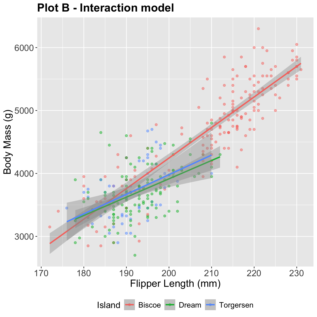
  • Slope (dream) : Holding flipper length constant, we expect, on average, a penguin from the Dream island to be 262g lighter than a penguin from Biscoe island.

The Interaction Model

The interaction model: different slopes for each island

bm_fl_island_int_fit <- linear_reg() |>
  fit(body_mass_g ~ flipper_length_mm * island, data = penguins)

tidy(bm_fl_island_int_fit) |> select(term, estimate)
# A tibble: 6 × 2
  term                              estimate
  <chr>                                <dbl>
1 (Intercept)                        -5464. 
2 flipper_length_mm                     48.5
3 islandDream                         3551. 
4 islandTorgersen                     3218. 
5 flipper_length_mm:islandDream        -19.4
6 flipper_length_mm:islandTorgersen    -17.4

. . .

\[ \begin{aligned} \widehat{body~mass} = -5464 + 48.5 \times flipper~length &+ 3551 \times Dream \\ &+ 3218 \times Torgersen \\ &- 19.4 \times flipper~length*Dream \\ &- 17.4 \times flipper~length*Torgersen \end{aligned} \]

Where do the three lines come from?

\[ \begin{aligned} \small\widehat{body~mass} = -5464 &+ 48.5 \times flipper~length \\ &+ 3551 \times Dream \\ &+ 3218 \times Torgersen \\ &- 19.4 \times flipper~length*Dream \\ &- 17.4 \times flipper~length*Torgersen \end{aligned} \]

If penguin is from Biscoe, Dream = 0 and Torgersen = 0:

. . .

\[ \begin{aligned} \widehat{body~mass} = -5464 &+ 48.5 \times flipper~length \end{aligned} \]

Where do the three lines come from?

\[ \begin{aligned} \small\widehat{body~mass} = -5464 &+ 48.5 \times flipper~length \\ &+ 3551 \times Dream \\ &+ 3218 \times Torgersen \\ &- 19.4 \times flipper~length*Dream \\ &- 17.4 \times flipper~length*Torgersen \end{aligned} \]

If penguin is from Dream, Dream = 1 and Torgersen = 0:

. . .

\[ \begin{aligned} \widehat{body~mass} &= (-5464 + 3551) + (48.5-19.4) \times flipper~length\\ &=-1913+29.1\times flipper~length. \end{aligned} \]

You try!

\[ \begin{aligned} \small\widehat{body~mass} = -5464 &+ 48.5 \times flipper~length \\ &+ 3551 \times Dream \\ &+ 3218 \times Torgersen \\ &- 19.4 \times flipper~length*Dream \\ &- 17.4 \times flipper~length*Torgersen \end{aligned} \] If penguin is from Torgersen, Dream = 0 and Torgersen = 1:

Interpretation

We can interpret each of the lines just as we would a simple linear regression, keeping in mind that we are only looking at penguins from one specific island.

. . .

Dream Penguins: \(\widehat{body~mass} = -1913 + 29.1 \times flipper~length\)

. . .

  • Intercept: For penguins from Dream island, a flipper length of 0 corresponds to, on average, a body mass of -1913 grams.

. . .

  • Slope: For penguins from Dream island, a 1mm increase in flipper length corresponds to, on average, a body mass increase of 29.1 grams.

Prediction

new_penguin <- tibble(
  flipper_length_mm = 200,
  island = "Torgersen"
)

predict(bm_fl_island_int_fit, new_data = new_penguin)
# A tibble: 1 × 1
  .pred
  <dbl>
1 3980.

\[ \widehat{body~mass} = (-5464 + 3218) + (48.5-17.4) \times 200. \]

A note on plotting…

This, we have done. It is what R naturally does when we use color = island!
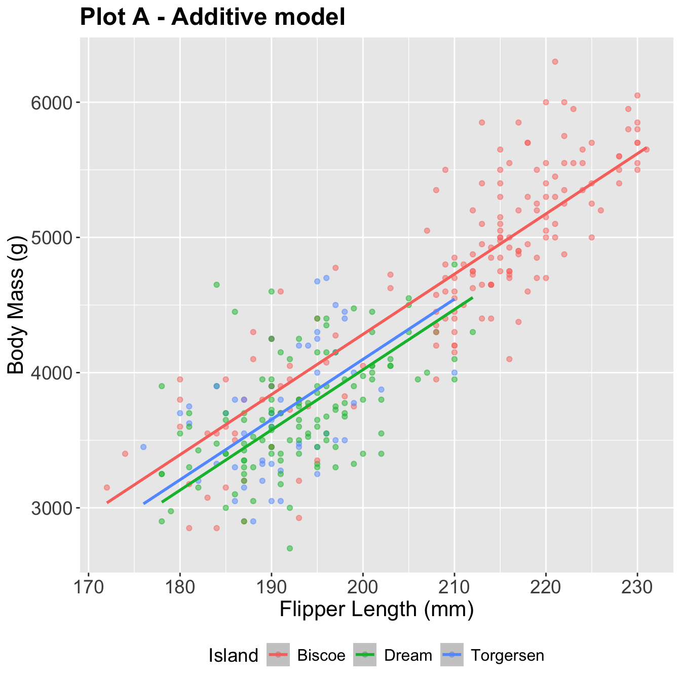
A note on plotting…

This, we have not! Here, we use the predicted y values (attained using augment) from an additive model in geom_smooth().

A note on plotting…

# Fit Model and use Augment

bm_fl_island_fit <- linear_reg() |>
  fit(body_mass_g ~ flipper_length_mm + island, data = penguins)
bm_fl_island_aug <- augment(bm_fl_island_fit, new_data = penguins)

# Additive model

ggplot(
  bm_fl_island_aug, 
  aes(x = flipper_length_mm, y = body_mass_g, color = island)
) +
  geom_point(alpha = 0.5) +
  geom_smooth(aes(y = .pred), method = "lm") +
  labs(
    title = "Plot A - Additive model",
    x = "Flipper Length (mm)",
    y = "Body Mass (g)",
    color = "Island"
  ) +
  theme(
    legend.position = "bottom",
    plot.title = element_text(size = 18, face = "bold"),
    axis.title = element_text(size = 16),
    axis.text = element_text(size = 14),
    legend.title = element_text(size = 14),
    legend.text = element_text(size = 12)
  )

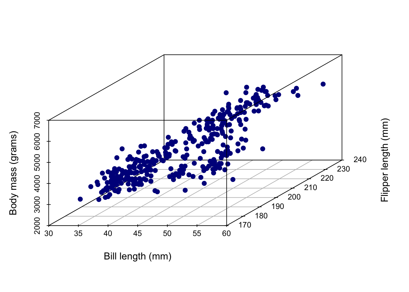
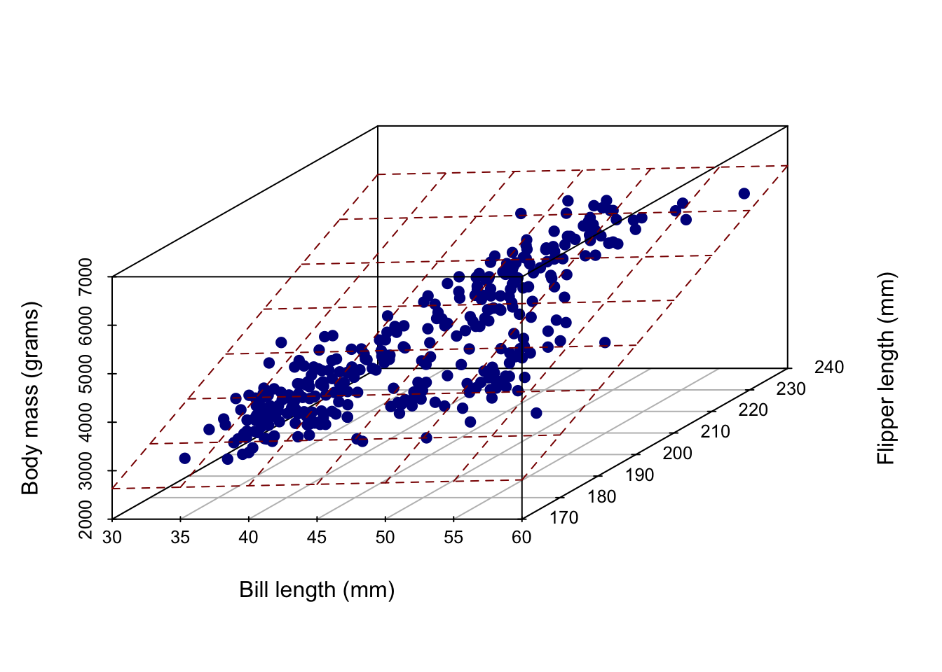
Multiple numeric predictors

Multiple Numerical Predictors

What if we want to use multiple numerical predictors to model a numerical outcome?

Example:

  • Using flipper length and bill length to predict body mass.

  • Using Rotten Tomato critic score + metacritic score to predict audience score

  • So many more!!

Multiple Numerical Predictors: Example

bm_fl_bl_fit <- linear_reg() |>
  fit(body_mass_g ~ flipper_length_mm * bill_length_mm, data = penguins)

tidy(bm_fl_bl_fit)
# A tibble: 4 × 5
  term                            estimate std.error statistic p.value
  <chr>                              <dbl>     <dbl>     <dbl>   <dbl>
1 (Intercept)                      5091.    2925.        1.74  8.27e-2
2 flipper_length_mm                  -7.31    15.0      -0.486 6.27e-1
3 bill_length_mm                   -229.      63.4      -3.61  3.47e-4
4 flipper_length_mm:bill_length_…     1.20     0.322     3.72  2.32e-4

. . .

\[ \small\widehat{body~mass}=-5736+48.1\times flipper~length+6\times bill~length \]

Multiple Numerical Predictors: Interpretation

\[ \small\widehat{body~mass}=-5736+48.1\times flipper~length+6\times bill~length \]

  • We predict that the body mass of a penguin with zero flipper length and zero bill length will be -5736 grams, on average (makes no sense);
  • Holding all other variables constant, for every additional millimeter in flipper length, we expect the body mass of penguins to be higher, on average, by 48.1 grams.
  • Holding all other variables constant, for every additional millimeter in bill length, we expect the body mass of penguins to be higher, on average, by 6 grams.

. . .

This is how we interpret additive models with as many predictors as we want!

Prediction

new_penguin <- tibble(
  flipper_length_mm = 200,
  bill_length_mm = 45
)

predict(bm_fl_bl_fit, new_data = new_penguin)
# A tibble: 1 × 1
  .pred
  <dbl>
1 4112.

\[ \widehat{body~mass}=-5736+48.1\times 200+6\times 45 \]

Picture? It’s not pretty…

2 predictors + 1 response = 3 dimensions. Ick!

Picture? It’s not pretty…

Instead of a line of best fit, it’s a plane of best fit. Double ick!

Multiple Numerical Predictors: With Interaction

bm_fl_bl_int_fit <- linear_reg() |>
  fit(body_mass_g ~ flipper_length_mm * bill_length_mm, data = penguins)

tidy(bm_fl_bl_int_fit)
# A tibble: 4 × 5
  term                            estimate std.error statistic p.value
  <chr>                              <dbl>     <dbl>     <dbl>   <dbl>
1 (Intercept)                      5091.    2925.        1.74  8.27e-2
2 flipper_length_mm                  -7.31    15.0      -0.486 6.27e-1
3 bill_length_mm                   -229.      63.4      -3.61  3.47e-4
4 flipper_length_mm:bill_length_…     1.20     0.322     3.72  2.32e-4

. . .

\[ \begin{aligned} \small \widehat{body~mass} =\;& 5090.5 - 7.3 \times flipper \\ &- 229.2 \times bill \\ &+ 1.2 \times flipper \times bill \end{aligned} \]

What does this model mean?

  • We still have an intercept and main effects for both flipper and bill. But now we also have an interaction term.

. . .

  • This means: the effect of flipper length depends on bill length, and vice versa.

. . .

  • In additive models: each variable has a fixed slope.
  • In interaction models: the slope of one predictor varies depending on the level of the other.

AE 13: Modelling House Prices