Midterm Review

Lecture 11

Published

May 30, 2025

Announcements

Office hours today from 1:00-3:00.
Be in class and lab on Monday!!!!

Review

group_by/summarize/mutate
joins
pivots

Computing summary stats

With summarize: condenses information into smaller result table
With mutate: adds a new column to the data
With groupby: results for each provided group

Sample Data

df <- tibble(
    C1 = c("A", "A", "A", "B", "B"),
    C2 = c("X", "Y", "X", "X", "Y"),
    C3 = 1:5
)

df

# A tibble: 5 × 3
  C1    C2       C3
  <chr> <chr> <int>
1 A     X         1
2 A     Y         2
3 A     X         3
4 B     X         4
5 B     Y         5

Mutate vs. Summarize

Compute the mean of C3.

df

# A tibble: 5 × 3
  C1    C2       C3
  <chr> <chr> <int>
1 A     X         1
2 A     Y         2
3 A     X         3
4 B     X         4
5 B     Y         5

df |>
  mutate(mean_3 = mean(C3))

# A tibble: 5 × 4
  C1    C2       C3 mean_3
  <chr> <chr> <int>  <dbl>
1 A     X         1      3
2 A     Y         2      3
3 A     X         3      3
4 B     X         4      3
5 B     Y         5      3

Mutate vs. Summarize

Compute the mean of C3.

df

# A tibble: 5 × 3
  C1    C2       C3
  <chr> <chr> <int>
1 A     X         1
2 A     Y         2
3 A     X         3
4 B     X         4
5 B     Y         5

df |>
  mutate(mean_3 = mean(C3))

# A tibble: 5 × 4
  C1    C2       C3 mean_3
  <chr> <chr> <int>  <dbl>
1 A     X         1      3
2 A     Y         2      3
3 A     X         3      3
4 B     X         4      3
5 B     Y         5      3

df |>
  summarise(mean_3 = mean(C3))

# A tibble: 1 × 1
  mean_3
   <dbl>
1      3

Grouping

Group by C1.

df

# A tibble: 5 × 3
  C1    C2       C3
  <chr> <chr> <int>
1 A     X         1
2 A     Y         2
3 A     X         3
4 B     X         4
5 B     Y         5

df |>
  group_by(C1)

# A tibble: 5 × 3
# Groups:   C1 [2]
  C1    C2       C3
  <chr> <chr> <int>
1 A     X         1
2 A     Y         2
3 A     X         3
4 B     X         4
5 B     Y         5

Grouping

Group by C1 and C2.

df

# A tibble: 5 × 3
  C1    C2       C3
  <chr> <chr> <int>
1 A     X         1
2 A     Y         2
3 A     X         3
4 B     X         4
5 B     Y         5

df |>
  group_by(C1, C2)

# A tibble: 5 × 3
# Groups:   C1, C2 [4]
  C1    C2       C3
  <chr> <chr> <int>
1 A     X         1
2 A     Y         2
3 A     X         3
4 B     X         4
5 B     Y         5

Mutate vs. Summarize (with grouping)

Compute the mean of C3 by value of C1.

df

# A tibble: 5 × 3
  C1    C2       C3
  <chr> <chr> <int>
1 A     X         1
2 A     Y         2
3 A     X         3
4 B     X         4
5 B     Y         5

df |>
  group_by(C1) |>
  mutate(mean_3 = mean(C3))

# A tibble: 5 × 4
# Groups:   C1 [2]
  C1    C2       C3 mean_3
  <chr> <chr> <int>  <dbl>
1 A     X         1    2  
2 A     Y         2    2  
3 A     X         3    2  
4 B     X         4    4.5
5 B     Y         5    4.5

Mutate vs. Summarize (with grouping)

Compute the mean of C3 by value of C1.

df

# A tibble: 5 × 3
  C1    C2       C3
  <chr> <chr> <int>
1 A     X         1
2 A     Y         2
3 A     X         3
4 B     X         4
5 B     Y         5

df |>
  group_by(C1) |>
  mutate(mean_3 = mean(C3))

# A tibble: 5 × 4
# Groups:   C1 [2]
  C1    C2       C3 mean_3
  <chr> <chr> <int>  <dbl>
1 A     X         1    2  
2 A     Y         2    2  
3 A     X         3    2  
4 B     X         4    4.5
5 B     Y         5    4.5

df |>
  group_by(C1) |>
  summarise(mean_3 = mean(C3))

# A tibble: 2 × 2
  C1    mean_3
  <chr>  <dbl>
1 A        2  
2 B        4.5

Mutate vs. Summarize (with grouping)

Compute the mean of C3 by value of C1 and C2.

df

# A tibble: 5 × 3
  C1    C2       C3
  <chr> <chr> <int>
1 A     X         1
2 A     Y         2
3 A     X         3
4 B     X         4
5 B     Y         5

df |>
  group_by(C1, C2) |>
  mutate(mean_3 = mean(C3))

# A tibble: 5 × 4
# Groups:   C1, C2 [4]
  C1    C2       C3 mean_3
  <chr> <chr> <int>  <dbl>
1 A     X         1      2
2 A     Y         2      2
3 A     X         3      2
4 B     X         4      4
5 B     Y         5      5

Mutate vs. Summarize (with grouping)

Compute the mean of C3 by value of C1 and C2.

df

# A tibble: 5 × 3
  C1    C2       C3
  <chr> <chr> <int>
1 A     X         1
2 A     Y         2
3 A     X         3
4 B     X         4
5 B     Y         5

df |>
  group_by(C1, C2) |>
  mutate(mean_3 = mean(C3))

# A tibble: 5 × 4
# Groups:   C1, C2 [4]
  C1    C2       C3 mean_3
  <chr> <chr> <int>  <dbl>
1 A     X         1      2
2 A     Y         2      2
3 A     X         3      2
4 B     X         4      4
5 B     Y         5      5

df |>
  group_by(C1, C2) |>
  summarise(mean_3 = mean(C3))

`summarise()` has grouped output by 'C1'. You can override using the
`.groups` argument.

# A tibble: 4 × 3
# Groups:   C1 [2]
  C1    C2    mean_3
  <chr> <chr>  <dbl>
1 A     X          2
2 A     Y          2
3 B     X          4
4 B     Y          5

More about summarize and grouping

df |>
  group_by(C1, C2) |>
  summarise(mean_3 = mean(C3))

`summarise()` has grouped output by 'C1'. You can override using the
`.groups` argument.

# A tibble: 4 × 3
# Groups:   C1 [2]
  C1    C2    mean_3
  <chr> <chr>  <dbl>
1 A     X          2
2 A     Y          2
3 B     X          4
4 B     Y          5

df |>
  group_by(C1, C2) |>
  summarise(mean_3 = mean(C3), 
            .groups = "drop")

# A tibble: 4 × 3
  C1    C2    mean_3
  <chr> <chr>  <dbl>
1 A     X          2
2 A     Y          2
3 B     X          4
4 B     Y          5

More about summarize and grouping

df |>
  group_by(C1, C2) |>
  summarise(mean_3 = mean(C3)) |>
  summarise(mean_again = mean(mean_3))

`summarise()` has grouped output by 'C1'. You can override using the
`.groups` argument.

# A tibble: 2 × 2
  C1    mean_again
  <chr>      <dbl>
1 A            2  
2 B            4.5

df |>
  group_by(C1, C2) |>
  summarise(mean_3 = mean(C3), 
            .groups = "drop")|>
  summarise(mean_again = mean(mean_3))

# A tibble: 1 × 1
  mean_again
       <dbl>
1       3.25

Joins

Joining: Example Data

df_X

id	X
1	X1
2	X2
3	X3

df_Y

id	Y
1	Y1
2	Y2
4	Y4

Joining: Left Join

df_X

id	X
1	X1
2	X2
3	X3

df_Y

id	Y
1	Y1
2	Y2
4	Y4

left_join(df_X, df_Y)

id	X	Y
1	X1	Y1
2	X2	Y2
3	X3	NA

Joining: Left Join

df_X

id	X
1	X1
2	X2
3	X3

df_Y

id	Y
1	Y1
2	Y2
4	Y4

left_join(df_X, df_Y)

id	X	Y
1	X1	Y1
2	X2	Y2
3	X3	NA

Joining: Right Join

df_X

id	X
1	X1
2	X2
3	X3

df_Y

id	Y
1	Y1
2	Y2
4	Y4

right_join(df_X, df_Y)

id	X	Y
1	X1	Y1
2	X2	Y2
4	NA	Y4

Joining: Right Join

df_X

id	X
1	X1
2	X2
3	X3

df_Y

id	Y
1	Y1
2	Y2
4	Y4

right_join(df_X, df_Y)

id	X	Y
1	X1	Y1
2	X2	Y2
4	NA	Y4

Joining: Full Join

df_X

id	X
1	X1
2	X2
3	X3

df_Y

id	Y
1	Y1
2	Y2
4	Y4

full_join(df_X, df_Y)

id	X	Y
1	X1	Y1
2	X2	Y2
3	X3	NA
4	NA	Y4

Joining: Full Join

df_X

id	X
1	X1
2	X2
3	X3

df_Y

id	Y
1	Y1
2	Y2
4	Y4

full_join(df_X, df_Y)

id	X	Y
1	X1	Y1
2	X2	Y2
3	X3	NA
4	NA	Y4

Joining: Inner Join

df_X

id	X
1	X1
2	X2
3	X3

df_Y

id	Y
1	Y1
2	Y2
4	Y4

inner_join(df_X, df_Y)

id	X	Y
1	X1	Y1
2	X2	Y2

Joining: Inner Join

df_X

id	X
1	X1
2	X2
3	X3

df_Y

id	Y
1	Y1
2	Y2
4	Y4

inner_join(df_X, df_Y)

id	X	Y
1	X1	Y1
2	X2	Y2

Joining: Semi Join

df_X

id	X
1	X1
2	X2
3	X3

df_Y

id	Y
1	Y1
2	Y2
4	Y4

semi_join(df_X, df_Y)

id	X
1	X1
2	X2

Joining: Semi Join

df_X

id	X
1	X1
2	X2
3	X3

df_Y

id	Y
1	Y1
2	Y2
4	Y4

semi_join(df_X, df_Y)

id	X
1	X1
2	X2

Joining: Anti Join

df_X

id	X
1	X1
2	X2
3	X3

df_Y

id	Y
1	Y1
2	Y2
4	Y4

anti_join(df_X, df_Y)

id	X
3	X3

Joining: Anti Join

df_X

id	X
1	X1
2	X2
3	X3

df_Y

id	Y
1	Y1
2	Y2
4	Y4

anti_join(df_X, df_Y)

id	X
3	X3

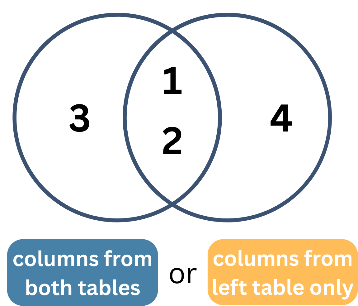
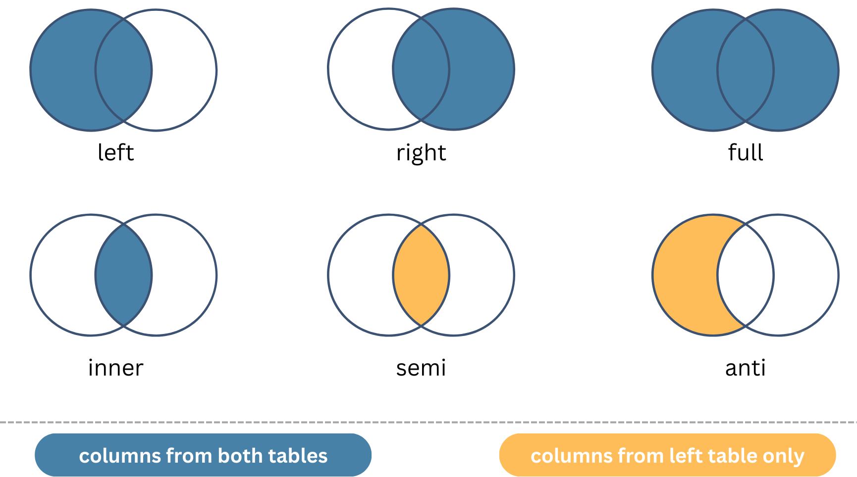
Summary of Join Types

Try it!

df_contacts

person	phone
Marie	1
Katie	2
John	3
John	4

df_texts

phone	texts
1	100
2	700
4	400
5	50

Remember…

Remember: sometimes we need to specify which columns we are joining with.

Review: Pivot Longer

How do we go from this…

# A tibble: 4 × 6
  degree `2011` `2012` `2013` `2014` `2015`
  <fct>   <dbl>  <dbl>  <dbl>  <dbl>  <dbl>
1 AB2        NA      1     NA     NA      4
2 AB          2      2      4      1      3
3 BS2         2      6      1     NA      5
4 BS          5      9      4     13     10

…to this?

# A tibble: 56 × 3
  degree  year     n
  <fct>  <dbl> <dbl>
1 AB2     2011    NA
2 AB2     2012     1
3 AB2     2013    NA
4 AB2     2014    NA
5 AB2     2015     4
# ℹ 51 more rows

Reverse It: Pivot Wider

How do we get back to this…

# A tibble: 4 × 6
  degree `2011` `2012` `2013` `2014` `2015`
  <fct>   <dbl>  <dbl>  <dbl>  <dbl>  <dbl>
1 AB2        NA      1     NA     NA      4
2 AB          2      2      4      1      3
3 BS2         2      6      1     NA      5
4 BS          5      9      4     13     10

… from this?

# A tibble: 56 × 3
  degree  year     n
  <fct>  <dbl> <dbl>
1 AB2     2011    NA
2 AB2     2012     1
3 AB2     2013    NA
4 AB2     2014    NA
5 AB2     2015     4
# ℹ 51 more rows

AE

Kahoot! See website for questions.