# A tibble: 5 × 2
      x y
  <dbl> <chr>
1     1 a
2     2 a
3     3 b
4     4 c
5 5 c Data Tidying
Lecture 5
Announcements/Reminders
You have lab today! Lab will be a little longer.
Tomorrow’s office hours are with Katie on Zoom.
Syllabus clarification re: lab attendance - you are allowed to miss one! But let me or Mary know it’s happening!
Outline
-
Last Time: Did more data transformation and exploratory data analysis.
- Look at the rest of AE-05!
Today: Learn about data tidying.
Assigment
How can we save the changes we make to a data frame?
Assignment
Let’s make a tiny data frame to use as an example:
Assignment
Do something and show me
df |>
  mutate(x = x * 2)
# A tibble: 5 × 2
x y
<dbl> <chr>
1 2 a
2 4 a
3 6 b
4 8 c
5 10 c df# A tibble: 5 × 2
x y
<dbl> <chr>
1 1 a
2 2 a
3 3 b
4 4 c
5 5 c Do something and save result
df <- df |>
mutate(x = x * 2)df# A tibble: 5 × 2
x y
<dbl> <chr>
1 2 a
2 4 a
3 6 b
4 8 c
5 10 c Assignment
Do something, save result, overwriting original
Assignment
Do something, save result, overwriting original when you shouldn’t
Assignment
Do something, save result, overwriting original
data frame
Assignment: when??
When should you assign results to a variable?
If you know you will want to use the result multiple times
We will tell you on the lab when we want you to assign a variable to a pipeline result vs. just show the pipeline
Caution
Be careful about overwriting the original data!!
Data tidying
Tidy data
“Tidy datasets are easy to manipulate, model and visualise, and have a specific structure: each variable is a column, each observation is a row, and each type of observational unit is a table.”
Tidy Data, https://vita.had.co.nz/papers/tidy-data.pdf
. . .
Note: “easy to manipulate” = “straightforward to manipulate”
Goal
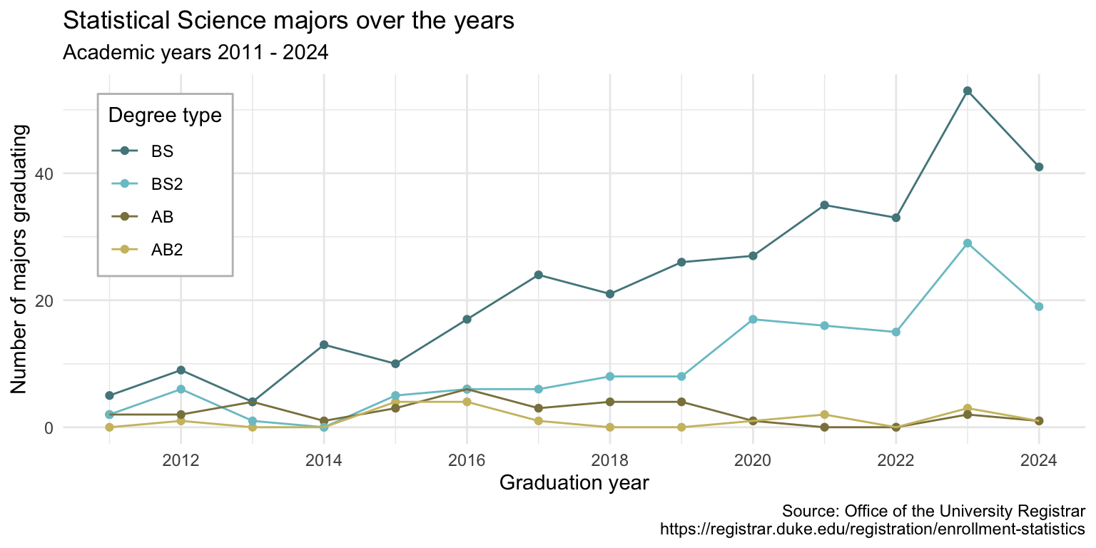
Visualize StatSci majors over the years!
Data
statsci <- read_csv("data/statsci.csv")Rows: 4 Columns: 15
── Column specification ──────────────────────────────────────────────
Delimiter: ","
chr (1): degree
dbl (14): 2011, 2012, 2013, 2014, 2015, 2016, 2017, 2018, 2019, 20...
ℹ Use `spec()` to retrieve the full column specification for this data.
ℹ Specify the column types or set `show_col_types = FALSE` to quiet this message.statsci# A tibble: 4 × 15
degree `2011` `2012` `2013` `2014` `2015` `2016` `2017` `2018`
<chr> <dbl> <dbl> <dbl> <dbl> <dbl> <dbl> <dbl> <dbl>
1 Statistical… NA 1 NA NA 4 4 1 NA
2 Statistical… 2 2 4 1 3 6 3 4
3 Statistical… 2 6 1 NA 5 6 6 8
4 Statistical… 5 9 4 13 10 17 24 21
# ℹ 6 more variables: `2019` <dbl>, `2020` <dbl>, `2021` <dbl>,
# `2022` <dbl>, `2023` <dbl>, `2024` <dbl>The first column (variable) is the
degree, and there are 4 possible degrees: BS (Bachelor of Science), BS2 (Bachelor of Science, 2nd major), AB (Bachelor of Arts), AB2 (Bachelor of Arts, 2nd major).The remaining columns show the number of students graduating with that major in a given academic year from 2011 to 2024.
Let’s plan!
In a perfect world, how would our data be formatted to create this plot? What do the columns need to be? What would go inside aes when we call ggplot?
The goal
We want to be able to write code that starts something like this:
But the data are not in a format that will allow us to do that.
The challenge
How do we go from this…
# A tibble: 4 × 8
  degree `2011` `2012` `2013` `2014` `2015` `2016` `2017`
  <fct>   <dbl>  <dbl>  <dbl>  <dbl>  <dbl>  <dbl>  <dbl>
1 AB2        NA      1     NA     NA      4      4      1
2 AB          2      2      4      1      3      6      3
3 BS2         2      6      1     NA      5      6      6
4 BS          5      9      4     13     10     17     24
…to this?
# A tibble: 56 × 3
   degree_type  year     n
   <fct>       <dbl> <dbl>
 1 AB2          2011     0
 2 AB2          2012     1
 3 AB2          2013     0
 4 AB2          2014     0
 5 AB2          2015     4
 6 AB2          2016     4
 7 AB2          2017     1
 8 AB2          2018     0
 9 AB2          2019     0
10 AB2          2020     1
11 AB2          2021     2
12 AB2          2022     0
13 AB2          2023     3
14 AB2          2024     1
15 AB           2011     2
16 AB           2012     2
# ℹ 40 more rows
. . .
With the command pivot_longer()!
pivot_longer()
Pivot the statsci data frame longer such that:
each row represents a degree type / year combination
yearandnumber of graduates for that year are columns in the data frame.
statsci |>
  pivot_longer(
    cols = -degree,
    names_to = "year",
    values_to = "n"
  )
# A tibble: 56 × 3
degree year n
<chr> <chr> <dbl>
1 Statistical Science (AB2) 2011 NA
2 Statistical Science (AB2) 2012 1
3 Statistical Science (AB2) 2013 NA
4 Statistical Science (AB2) 2014 NA
5 Statistical Science (AB2) 2015 4
6 Statistical Science (AB2) 2016 4
7 Statistical Science (AB2) 2017 1
8 Statistical Science (AB2) 2018 NA
9 Statistical Science (AB2) 2019 NA
10 Statistical Science (AB2) 2020 1
# ℹ 46 more rowsyear
What is the type of the year variaBle? Why? What should it be?
. . .
It’s a character (
chr) variable because the information came from the column names of the original data frameR cannot know that these words represent years.
The variable type should be numeric.