AE 16: Houses in Duke Forest
Suggested answers
In this application exercise, we use bootstrapping to construct confidence intervals.
Packages
We will use tidyverse and tidymodels for data exploration and modeling, respectively, and the openintro package for the data, and the knitr package for formatting tables.
Data
The data are on houses that were sold in the Duke Forest neighborhood of Durham, NC around November 2020. It was originally scraped from Zillow, and can be found in the duke_forest data set in the openintro R package.
glimpse(duke_forest)Rows: 98
Columns: 13
$ address <chr> "1 Learned Pl, Durham, NC 27705", "1616 Pinecrest Rd, Durha…
$ price <dbl> 1520000, 1030000, 420000, 680000, 428500, 456000, 1270000, …
$ bed <dbl> 3, 5, 2, 4, 4, 3, 5, 4, 4, 3, 4, 4, 3, 5, 4, 5, 3, 4, 4, 3,…
$ bath <dbl> 4.0, 4.0, 3.0, 3.0, 3.0, 3.0, 5.0, 3.0, 5.0, 2.0, 3.0, 3.0,…
$ area <dbl> 6040, 4475, 1745, 2091, 1772, 1950, 3909, 2841, 3924, 2173,…
$ type <chr> "Single Family", "Single Family", "Single Family", "Single …
$ year_built <dbl> 1972, 1969, 1959, 1961, 2020, 2014, 1968, 1973, 1972, 1964,…
$ heating <chr> "Other, Gas", "Forced air, Gas", "Forced air, Gas", "Heat p…
$ cooling <fct> central, central, central, central, central, central, centr…
$ parking <chr> "0 spaces", "Carport, Covered", "Garage - Attached, Covered…
$ lot <dbl> 0.97, 1.38, 0.51, 0.84, 0.16, 0.45, 0.94, 0.79, 0.53, 0.73,…
$ hoa <chr> NA, NA, NA, NA, NA, NA, NA, NA, NA, NA, NA, NA, NA, NA, NA,…
$ url <chr> "https://www.zillow.com/homedetails/1-Learned-Pl-Durham-NC-…Bootstrap confidence interval
1. Calculate the observed fit (slope)
observed_fit <- duke_forest |>
  specify(price ~ area) |>
  fit()

observed_fit
# A tibble: 2 × 2
term estimate
<chr> <dbl>
1 intercept 116652.
2 area 159.2. Take n bootstrap samples and fit models to each one.
Fill in the code, then set eval: true .
n = 100
set.seed(1234)

boot_fits <- duke_forest |>
  specify(price ~ area) |>
  generate(reps = n, type = "bootstrap") |>
  fit()

boot_fits
# A tibble: 200 × 3
# Groups: replicate [100]
replicate term estimate
<int> <chr> <dbl>
1 1 intercept 177388.
2 1 area 125.
3 2 intercept 161078.
4 2 area 150.
5 3 intercept 202354.
6 3 area 118.
7 4 intercept 120750.
8 4 area 162.
9 5 intercept 52127.
10 5 area 180.
# ℹ 190 more rowsWhy do we set a seed before taking the bootstrap samples?
Make a histogram of the bootstrap samples to visualize the bootstrap distribution.
boot_fits |>
  filter(term  == "area") |>
  ggplot(aes(x = estimate )) +
  geom_histogram()
`stat_bin()` using `bins = 30`. Pick better value with `binwidth`.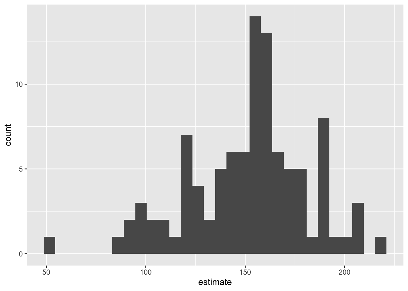
3. Compute the 95% confidence interval as the middle 95% of the bootstrap distribution
get_confidence_interval(
  boot_fits,
  point_estimate = observed_fit,
  level = 0.95,
  type = "percentile"
)
# A tibble: 2 × 3
term lower_ci upper_ci
<chr> <dbl> <dbl>
1 area 92.4 206.
2 intercept 7014. 285255.Changing confidence level
Modify the code from Step 3 to create a 90% confidence interval.
get_confidence_interval(
  boot_fits,
  point_estimate = observed_fit,
  level = 0.9,
  type = "percentile"
)
# A tibble: 2 × 3
term lower_ci upper_ci
<chr> <dbl> <dbl>
1 area 96.1 197.
2 intercept 20626. 268049.Modify the code from Step 3 to create a 99% confidence interval.
get_confidence_interval(
  boot_fits,
  point_estimate = observed_fit,
  level = 0.99,
  type = "percentile"
)
# A tibble: 2 × 3
term lower_ci upper_ci
<chr> <dbl> <dbl>
1 area 69.7 214.
2 intercept -25879. 351614.Which confidence level produces the most accurate confidence interval (90%, 95%, 99%)?
Which confidence level produces the most precise confidence interval (90%, 95%, 99%)?
If we want to be very certain that we capture the population parameter, should we use a wider or a narrower interval? What drawbacks are associated with using a wider interval?
The most accurate is the 90% interval - as the widest interval, it is most likely to capture the true parameter. The most precise is the 99% interval - it is the narrowest. A wider interval makes it more likely that we capture the true parameter but can make interpretation less meaningful.