AE 15: Forest classification
In this application exercise, we will
- Split our data into testing and training
- Fit logistic regression regression models to testing data to classify outcomes
- Evaluate performance of models on testing data
We will use tidyverse and tidymodels for data exploration and modeling, respectively, and the forested package for the data.
Remember from the lecture that the forested dataset contains information on whether a plot is forested (Yes) or not (No) as well as numerical and categorical features of that plot.
glimpse(forested)Rows: 7,107
Columns: 19
$ forested <fct> Yes, Yes, No, Yes, Yes, Yes, Yes, Yes, Yes, Yes, Yes,…
$ year <dbl> 2005, 2005, 2005, 2005, 2005, 2005, 2005, 2005, 2005,…
$ elevation <dbl> 881, 113, 164, 299, 806, 736, 636, 224, 52, 2240, 104…
$ eastness <dbl> 90, -25, -84, 93, 47, -27, -48, -65, -62, -67, 96, -4…
$ northness <dbl> 43, 96, 53, 34, -88, -96, 87, -75, 78, -74, -26, 86, …
$ roughness <dbl> 63, 30, 13, 6, 35, 53, 3, 9, 42, 99, 51, 190, 95, 212…
$ tree_no_tree <fct> Tree, Tree, Tree, No tree, Tree, Tree, No tree, Tree,…
$ dew_temp <dbl> 0.04, 6.40, 6.06, 4.43, 1.06, 1.35, 1.42, 6.39, 6.50,…
$ precip_annual <dbl> 466, 1710, 1297, 2545, 609, 539, 702, 1195, 1312, 103…
$ temp_annual_mean <dbl> 6.42, 10.64, 10.07, 9.86, 7.72, 7.89, 7.61, 10.45, 10…
$ temp_annual_min <dbl> -8.32, 1.40, 0.19, -1.20, -5.98, -6.00, -5.76, 1.11, …
$ temp_annual_max <dbl> 12.91, 15.84, 14.42, 15.78, 13.84, 14.66, 14.23, 15.3…
$ temp_january_min <dbl> -0.08, 5.44, 5.72, 3.95, 1.60, 1.12, 0.99, 5.54, 6.20…
$ vapor_min <dbl> 78, 34, 49, 67, 114, 67, 67, 31, 60, 79, 172, 162, 70…
$ vapor_max <dbl> 1194, 938, 754, 1164, 1254, 1331, 1275, 944, 892, 549…
$ canopy_cover <dbl> 50, 79, 47, 42, 59, 36, 14, 27, 82, 12, 74, 66, 83, 6…
$ lon <dbl> -118.6865, -123.0825, -122.3468, -121.9144, -117.8841…
$ lat <dbl> 48.69537, 47.07991, 48.77132, 45.80776, 48.07396, 48.…
$ land_type <fct> Tree, Tree, Tree, Tree, Tree, Tree, Non-tree vegetati…Spending your data
Split your data into testing and training in a reproducible manner and display the split object.
set.seed(1234)
forested_split <- initial_split(forested)
forested_split
<Training/Testing/Total>
<5330/1777/7107>Now, save your training and testing data as their own data frames.
forested_train <- training(forested_split)
forested_test <- testing(forested_split)
Exploratory data analysis
Create some visualizations to explore the data! This can help you determine which predictors you want to include in your model.
Note: Pay attention to which dataset you use for your exploration.
This is a plot that explores latitude and longitude - it’s different from anything we have seen so far!
ggplot(forested_train, aes(x = lon, y = lat, color = forested)) +
  geom_point(alpha = 0.7) +
  scale_color_manual(values = c("Yes" = "forestgreen", "No" = "gold2")) +
  theme_minimal()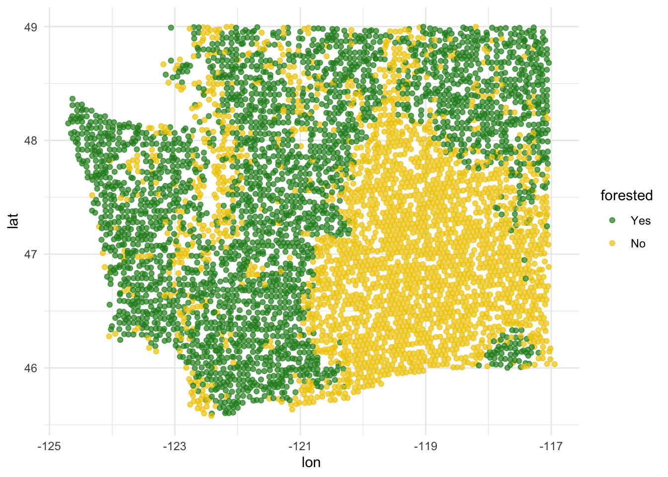
# add some other plots here!

ggplot(forested_train, aes(x = tree_no_tree, fill = forested)) +
  geom_bar(position = "fill")+
  scale_fill_manual(values = c("Yes" = "forestgreen", "No" = "gold2")) +
  theme_minimal()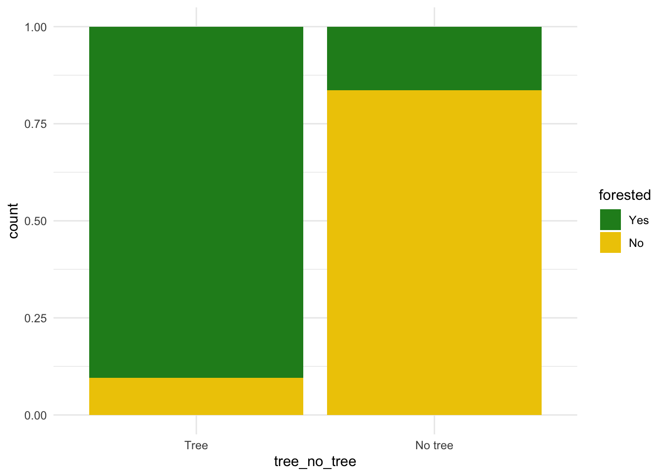
ggplot(forested_train, aes(x = temp_annual_mean, color = forested)) +
  geom_density() +
  scale_color_manual(values = c("Yes" = "forestgreen", "No" = "gold2")) +
  theme_minimal()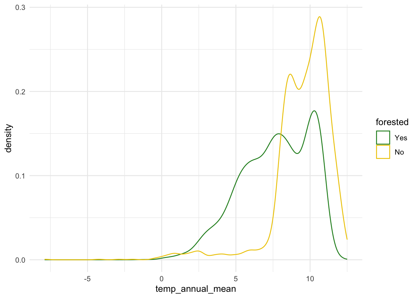
Model 1: Custom choice of predictors
Fit
Fit a model for classifying plots as forested or not based on a subset of predictors of your choice. Name the model forested_custom_fit and display a tidy output of the model.
forested_custom_fit <- logistic_reg() |>
  fit(forested ~ lat + lon + tree_no_tree + temp_annual_mean,
      data = forested_train)

tidy(forested_custom_fit)
# A tibble: 5 × 5
term estimate std.error statistic p.value
<chr> <dbl> <dbl> <dbl> <dbl>
1 (Intercept) 44.7 4.13 10.8 2.93e- 27
2 lat -0.285 0.0544 -5.25 1.51e- 7
3 lon 0.298 0.0242 12.3 6.63e- 35
4 tree_no_treeNo tree 3.35 0.0920 36.4 6.65e-290
5 temp_annual_mean 0.334 0.0219 15.2 1.94e- 52Predict
Predict for the testing data using this model.
forested_custom_aug <- augment(forested_custom_fit, new_data = forested_test)

forested_custom_aug
# A tibble: 1,777 × 22
.pred_class .pred_Yes .pred_No forested year elevation eastness northness
<fct> <dbl> <dbl> <fct> <dbl> <dbl> <dbl> <dbl>
1 Yes 0.878 0.122 Yes 2005 113 -25 96
2 Yes 0.833 0.167 Yes 2005 736 -27 -96
3 Yes 0.855 0.145 Yes 2005 224 -65 -75
4 Yes 0.955 0.0451 Yes 2003 1031 -49 86
5 Yes 0.716 0.284 No 2005 1713 -66 75
6 Yes 0.982 0.0181 Yes 2014 1612 30 -95
7 No 0.0781 0.922 No 2014 507 44 -89
8 Yes 0.885 0.115 Yes 2014 940 -93 35
9 Yes 0.653 0.347 No 2014 246 22 -97
10 No 0.0890 0.911 No 2014 419 86 -49
# ℹ 1,767 more rows
# ℹ 14 more variables: roughness <dbl>, tree_no_tree <fct>, dew_temp <dbl>,
# precip_annual <dbl>, temp_annual_mean <dbl>, temp_annual_min <dbl>,
# temp_annual_max <dbl>, temp_january_min <dbl>, vapor_min <dbl>,
# vapor_max <dbl>, canopy_cover <dbl>, lon <dbl>, lat <dbl>, land_type <fct>Evaluate
Calculate the false positive and false negative rates for the testing data using this model.
forested_custom_aug |>
  count(.pred_class, forested) |>
  arrange(forested) |>
  group_by(forested) |>
  mutate(
    p = round(n / sum(n), 2),
    decision = case_when(
      .pred_class == "Yes" & forested == "Yes" ~ "True positive",
      .pred_class == "Yes" & forested == "No" ~ "False positive",
      .pred_class == "No" & forested == "Yes" ~ "False negative",
      .pred_class == "No" & forested == "No" ~ "True negative"
    )
  )
# A tibble: 4 × 5
# Groups: forested [2]
.pred_class forested n p decision
<fct> <fct> <int> <dbl> <chr>
1 Yes Yes 864 0.9 True positive
2 No Yes 98 0.1 False negative
3 Yes No 123 0.15 False positive
4 No No 692 0.85 True negative Another commonly used display of this information is a confusion matrix. Create this using the conf_mat() function.
conf_mat(
  forested_custom_aug,
  truth = forested,
  estimate = .pred_class
)
Truth
Prediction Yes No
Yes 864 123
No 98 692Sensitivity, specificity, ROC curve
Calculate sensitivity and specificity and draw the ROC curve.
forested_custom_roc <- roc_curve(forested_custom_aug,
                                 truth = forested,  # column with truth
                                 .pred_Yes, # column with y = 1 preds
                                 event_level = "first") # factor level for y = 1

forested_custom_roc
# A tibble: 1,779 × 3
.threshold specificity sensitivity
<dbl> <dbl> <dbl>
1 -Inf 0 1
2 0.0179 0 1
3 0.0187 0.00123 1
4 0.0195 0.00245 1
5 0.0199 0.00368 1
6 0.0219 0.00491 1
7 0.0282 0.00613 1
8 0.0287 0.00736 1
9 0.0294 0.00859 1
10 0.0295 0.00982 1
# ℹ 1,769 more rowsggplot(forested_custom_roc, aes(x = 1 - specificity, y = sensitivity)) +
geom_path() + # draws line
geom_abline(lty = 3) + # x = y line
coord_equal() # makes square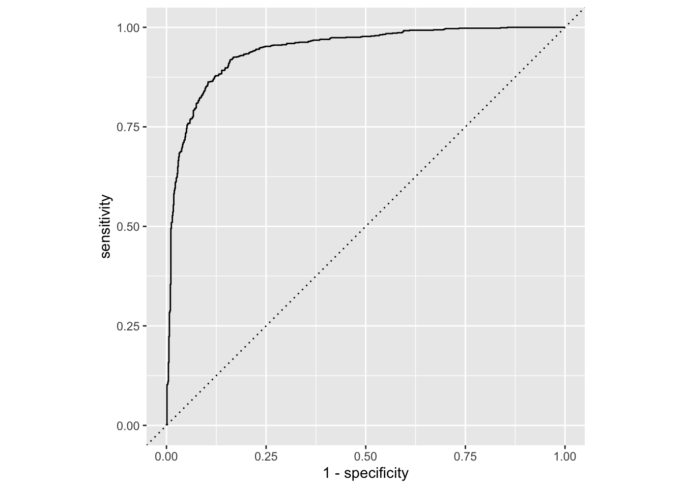
Model 2: All predictors
Fit
Fit a model for classifying plots as forested or not based on all predictors available. Name the model forested_full_fit and display a tidy output of the model.
forested_full_fit <- logistic_reg() |>
  fit(forested ~ ., data = forested_train)

tidy(forested_full_fit)
# A tibble: 20 × 5
term estimate std.error statistic p.value
<chr> <dbl> <dbl> <dbl> <dbl>
1 (Intercept) -12.1 32.6 -0.371 7.11e- 1
2 year 0.00456 0.0152 0.299 7.65e- 1
3 elevation -0.00277 0.000639 -4.33 1.47e- 5
4 eastness -0.000910 0.000734 -1.24 2.15e- 1
5 northness 0.00208 0.000745 2.79 5.26e- 3
6 roughness -0.00399 0.00146 -2.73 6.29e- 3
7 tree_no_treeNo tree 1.25 0.136 9.23 2.61e-20
8 dew_temp -0.125 0.176 -0.712 4.76e- 1
9 precip_annual -0.0000895 0.000100 -0.895 3.71e- 1
10 temp_annual_mean -7.30 12.4 -0.587 5.57e- 1
11 temp_annual_min 0.819 0.103 7.93 2.20e-15
12 temp_annual_max 2.59 6.22 0.417 6.77e- 1
13 temp_january_min 3.34 6.21 0.538 5.91e- 1
14 vapor_min 0.00000990 0.00353 0.00280 9.98e- 1
15 vapor_max 0.00925 0.00132 7.00 2.62e-12
16 canopy_cover -0.0446 0.00366 -12.2 4.18e-34
17 lon -0.0953 0.0559 -1.71 8.80e- 2
18 lat 0.0748 0.109 0.683 4.94e- 1
19 land_typeNon-tree vegetation -0.735 0.282 -2.61 9.05e- 3
20 land_typeTree -1.58 0.297 -5.33 9.93e- 8Predict
Predict for the testing data using this model.
forested_full_aug <- augment(forested_full_fit, new_data = forested_test)

forested_full_aug
# A tibble: 1,777 × 22
.pred_class .pred_Yes .pred_No forested year elevation eastness northness
<fct> <dbl> <dbl> <fct> <dbl> <dbl> <dbl> <dbl>
1 Yes 0.930 0.0700 Yes 2005 113 -25 96
2 Yes 0.918 0.0822 Yes 2005 736 -27 -96
3 No 0.428 0.572 Yes 2005 224 -65 -75
4 Yes 0.972 0.0280 Yes 2003 1031 -49 86
5 Yes 0.633 0.367 No 2005 1713 -66 75
6 Yes 0.980 0.0201 Yes 2014 1612 30 -95
7 No 0.0436 0.956 No 2014 507 44 -89
8 Yes 0.845 0.155 Yes 2014 940 -93 35
9 No 0.0141 0.986 No 2014 246 22 -97
10 No 0.0386 0.961 No 2014 419 86 -49
# ℹ 1,767 more rows
# ℹ 14 more variables: roughness <dbl>, tree_no_tree <fct>, dew_temp <dbl>,
# precip_annual <dbl>, temp_annual_mean <dbl>, temp_annual_min <dbl>,
# temp_annual_max <dbl>, temp_january_min <dbl>, vapor_min <dbl>,
# vapor_max <dbl>, canopy_cover <dbl>, lon <dbl>, lat <dbl>, land_type <fct>Evaluate
Calculate the false positive and false negative rates for the testing data using this model.
forested_full_aug |>
  count(.pred_class, forested) |>
  arrange(forested) |>
  group_by(forested) |>
  mutate(
    p = round(n / sum(n), 2),
    decision = case_when(
      .pred_class == "Yes" & forested == "Yes" ~ "True positive",
      .pred_class == "Yes" & forested == "No" ~ "False positive",
      .pred_class == "No" & forested == "Yes" ~ "False negative",
      .pred_class == "No" & forested == "No" ~ "True negative"
    )
  )
# A tibble: 4 × 5
# Groups: forested [2]
.pred_class forested n p decision
<fct> <fct> <int> <dbl> <chr>
1 Yes Yes 876 0.91 True positive
2 No Yes 86 0.09 False negative
3 Yes No 85 0.1 False positive
4 No No 730 0.9 True negative Sensitivity, specificity, ROC curve
Calculate sensitivity and specificity and draw the ROC curve.
forested_full_roc <- roc_curve(forested_full_aug,
                               truth = forested,  # column with truth
                                 .pred_Yes, # column with y = 1 preds
                                 event_level = "first" # factor level for y = 1
                               )

forested_full_roc
# A tibble: 1,779 × 3
.threshold specificity sensitivity
<dbl> <dbl> <dbl>
1 -Inf 0 1
2 0.00106 0 1
3 0.00107 0.00123 1
4 0.00217 0.00245 1
5 0.00287 0.00368 1
6 0.00290 0.00491 1
7 0.00290 0.00613 1
8 0.00309 0.00736 1
9 0.00321 0.00859 1
10 0.00323 0.00982 1
# ℹ 1,769 more rowsggplot(forested_full_roc, aes(x = 1 - specificity, y = sensitivity)) +
geom_path() + # draws line
geom_abline(lty = 3) + # x = y line
coord_equal() #makes plot square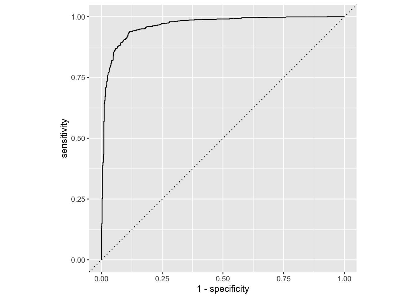
Model 1 vs. Model 2
Plot both ROC curves and articulate how you would use them to compare these models.
First, add a column to each roc data.
Next, combine data.
roc_combined <- bind_rows(forested_custom_roc, forested_full_roc) Now, plot!
roc_combined |>
  ggplot(aes(x = 1 - specificity, y = sensitivity, color = model)) +
  geom_path() + # draws line
  geom_abline(lty = 3) + # adds x = y line
  coord_equal() # makes square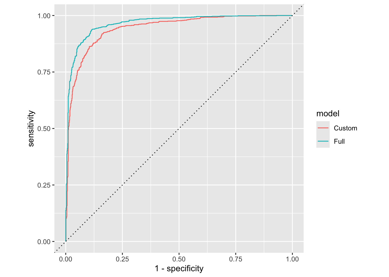
The full model looks better. We can quantify this comparison with the area under the curve:
# same as roc_curve, but roc_auc

full_roc_auc <- roc_auc (
  forested_full_aug,
  truth = forested,
  .pred_Yes,
  event_level = "first"
)

# same as roc_curve, but roc_auc
custom_roc_auc <- roc_auc (
  forested_custom_aug,
  truth = forested,
  .pred_Yes,
  event_level = "first"
)

full_roc_auc
# A tibble: 1 × 3
.metric .estimator .estimate
<chr> <chr> <dbl>
1 roc_auc binary 0.965custom_roc_auc# A tibble: 1 × 3
.metric .estimator .estimate
<chr> <chr> <dbl>
1 roc_auc binary 0.943