AE 13: Modeling housing prices

Application exercise

In this application exercise we will be studying housing prices. The dataset is a cleaned version of publicly available real estate data. We will use tidyverse and tidymodels for data exploration and modeling, respectively.

library(tidyverse)
library(tidymodels)
library(modeldata)

We will use the ames_housing dataset from the modeldata package.

Before we use the dataset, we’ll make a few transformations to it.

Your turn: Review the code below with your neighbors and write a summary of the data transformation pipeline.

data(ames)
housing <- ames |>
  select(Sale_Price, Gr_Liv_Area, Bldg_Type, Bedroom_AbvGr, Paved_Drive, Exter_Cond) |>
  mutate(home_type = fct_collapse(Bldg_Type,
    "House" = c("OneFam", "TwnhsE"),
    "Townhouse" = "Twnhs",
    "Duplex" = "Duplex"
  )) |>
  select(-Bldg_Type) |>
  rename(price = Sale_Price, sqft = Gr_Liv_Area, bedrooms = Bedroom_AbvGr) |>
  filter(home_type %in% c("House", "Townhouse", "Duplex"))

Here is a glimpse at the data:

glimpse(housing)

Rows: 2,868
Columns: 6
$ price       <int> 215000, 105000, 172000, 244000, 189900, 195500, 213500, 19…
$ sqft        <int> 1656, 896, 1329, 2110, 1629, 1604, 1338, 1280, 1616, 1804,…
$ bedrooms    <int> 3, 2, 3, 3, 3, 3, 2, 2, 2, 3, 3, 3, 3, 2, 1, 4, 4, 1, 2, 3…
$ Paved_Drive <fct> Partial_Pavement, Paved, Paved, Paved, Paved, Paved, Paved…
$ Exter_Cond  <fct> Typical, Typical, Typical, Typical, Typical, Typical, Typi…
$ home_type   <fct> House, House, House, House, House, House, House, House, Ho…

Get to know the data

Your turn: What is a typical house price in this dataset? What are some common square footage sizes? What types of homes are most common? Additionally, explore at least 1-2 other features that could be interesting. Share your findings!

# add code here

Price vs. square footage

How can we use square footage to model/predict pricing? Here is the model:

price_sqft_fit <- linear_reg() |>
  fit(price ~ sqft, data = housing)

tidy(price_sqft_fit)

# A tibble: 2 × 5
  term        estimate std.error statistic  p.value
  <chr>          <dbl>     <dbl>     <dbl>    <dbl>
1 (Intercept)   11430.   3271.        3.49 0.000482
2 sqft            114.      2.07     55.0  0

And here is the model visualized:

ggplot(housing, aes(x = sqft, y = price)) +
  geom_point(alpha = 0.4) +
  geom_smooth(method = "lm")

`geom_smooth()` using formula = 'y ~ x'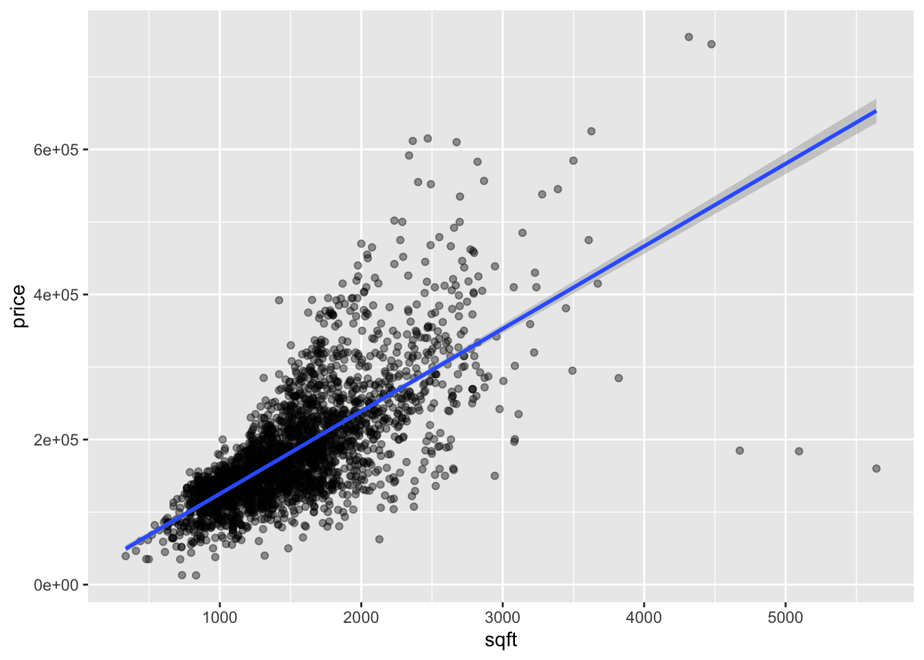

Your turn: Write the equation of the model in mathematical notation. Then, interpret the intercept and slope.

Price vs. home type

price_type_fit <- linear_reg() |>
  fit(price ~ home_type, data = housing)

tidy(price_type_fit)

# A tibble: 3 × 5
  term               estimate std.error statistic  p.value
  <chr>                 <dbl>     <dbl>     <dbl>    <dbl>
1 (Intercept)         185469.     1537.    121.   0       
2 home_typeDuplex     -45661.     7746.     -5.89 4.20e- 9
3 home_typeTownhouse  -49535.     8036.     -6.16 8.06e-10

Your turn: Write the equation of the model in mathematical notation. Then, interpret the intercept and each coefficient in context.

Price vs. square footage and home type

Now, let’s make some model that use both variables!

Main effects model

The main effects model is another name for the additive model. We fit the models below and wrote the model in math notation.

price_main_fit <- linear_reg() |>
  fit(price ~ sqft + home_type, data = housing)

tidy(price_main_fit)

# A tibble: 4 × 5
  term               estimate std.error statistic  p.value
  <chr>                 <dbl>     <dbl>     <dbl>    <dbl>
1 (Intercept)          13395.   3225.        4.15 3.38e- 5
2 sqft                   115.      2.03     56.5  0       
3 home_typeDuplex     -63251.   5338.      -11.8  1.19e-31
4 home_typeTownhouse  -20306.   5552.       -3.66 2.60e- 4

\[ \widehat{price} = 13394.8 + 114.5 \times sqft - 20306 \times Townhouse - 63251 \times Duplex \]

Task: Write the model equations for each home type. Provide interpretations of the coefficients.

Add answer here.

Interaction effects model

Now, we will fit an interaction effects model.

Task: Write code to fit an interaction effects model predicting price from square feet and home type.

#add code here

Task: Write the model output using mathematical notation.

Add answer here.

Task: Write the model equations for each home type.

Add answer here.

Model Comparison

So, we fit multiple models - how do we know which one is better?

We will dive into this tomorrow, but there is a value called adjusted \(R^2\) that lets us compare models. Higher values are better, lower are worse. You can glance() at a model fit to see the adjusted \(R^2\) values.

Which model is the best fit? Which is the worst?

# add code here

One more model?

Task: Try adding one more variable to your chosen model from above. Does it make a difference in adjusted \(R^2\)?

# add code here