AE 13: Modeling housing prices

Suggested answers

Important

These are suggested answers. This document should be used as reference only, it’s not designed to be an exhaustive key.

In this application exercise we will be studying housing prices. The dataset is a cleaned version of publicly available real estate data. We will use tidyverse and tidymodels for data exploration and modeling, respectively.

library(tidyverse)
library(tidymodels)
library(modeldata)

We will use the ames_housing dataset from the modeldata package.

Before we use the dataset, we’ll make a few transformations to it.

• Your turn: Review the code below with your neighbor and write a summary of the data transformation pipeline.

Add response here.

data(ames)
housing <- ames |>
  select(Sale_Price, Gr_Liv_Area, Bldg_Type, Bedroom_AbvGr, Paved_Drive, Exter_Cond) |>
  mutate(home_type = fct_collapse(Bldg_Type,
    "House" = c("OneFam", "TwnhsE"),
    "Townhouse" = "Twnhs",
    "Duplex" = "Duplex"
  )) |>
  select(-Bldg_Type) |>
  rename(price = Sale_Price, sqft = Gr_Liv_Area, bedrooms = Bedroom_AbvGr) |>
  filter(home_type %in% c("House", "Townhouse", "Duplex"))

Here is a glimpse at the data:

glimpse(housing)

Rows: 2,868
Columns: 6
$ price       <int> 215000, 105000, 172000, 244000, 189900, 195500, 213500, 19…
$ sqft        <int> 1656, 896, 1329, 2110, 1629, 1604, 1338, 1280, 1616, 1804,…
$ bedrooms    <int> 3, 2, 3, 3, 3, 3, 2, 2, 2, 3, 3, 3, 3, 2, 1, 4, 4, 1, 2, 3…
$ Paved_Drive <fct> Partial_Pavement, Paved, Paved, Paved, Paved, Paved, Paved…
$ Exter_Cond  <fct> Typical, Typical, Typical, Typical, Typical, Typical, Typi…
$ home_type   <fct> House, House, House, House, House, House, House, House, Ho…

Get to know the data

• Your turn: What is a typical house price in this dataset? What are some common square footage sizes? What types of homes are most common? Additionally, explore at least 1-2 other features that could be interesting. Share your findings!

ggplot(housing, aes(x = price)) +
  geom_histogram(binwidth = 20000)
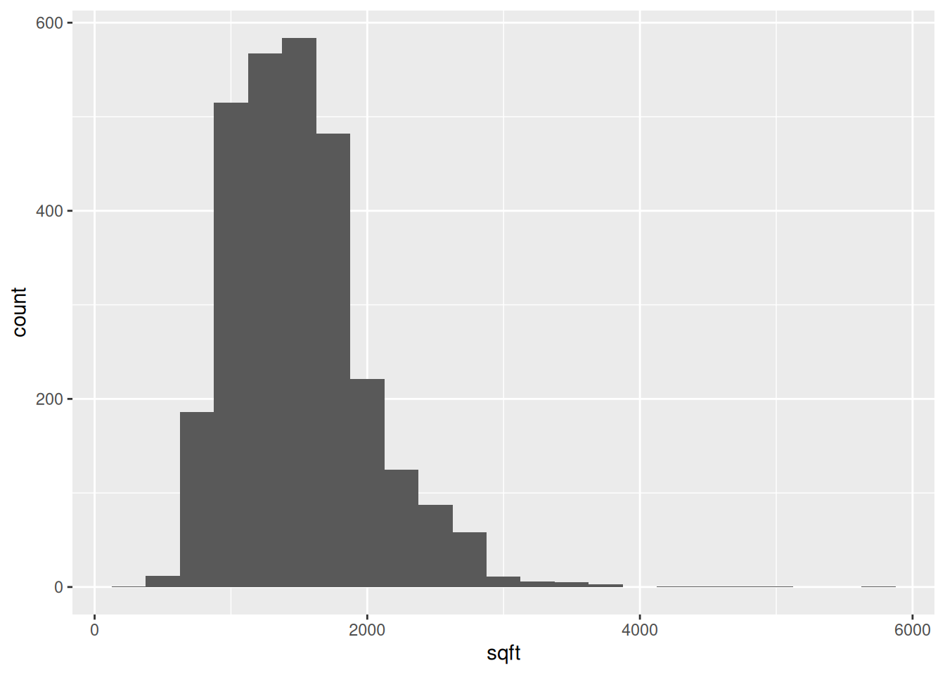
ggplot(housing, aes(x = sqft)) +
  geom_histogram(binwidth = 250)
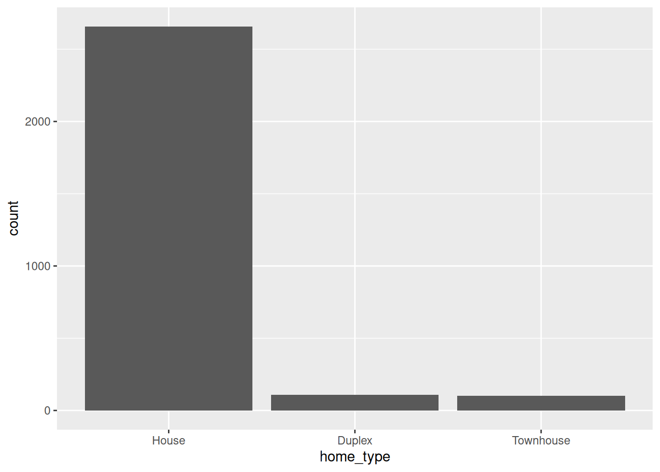
ggplot(housing, aes(x = home_type)) +
  geom_bar()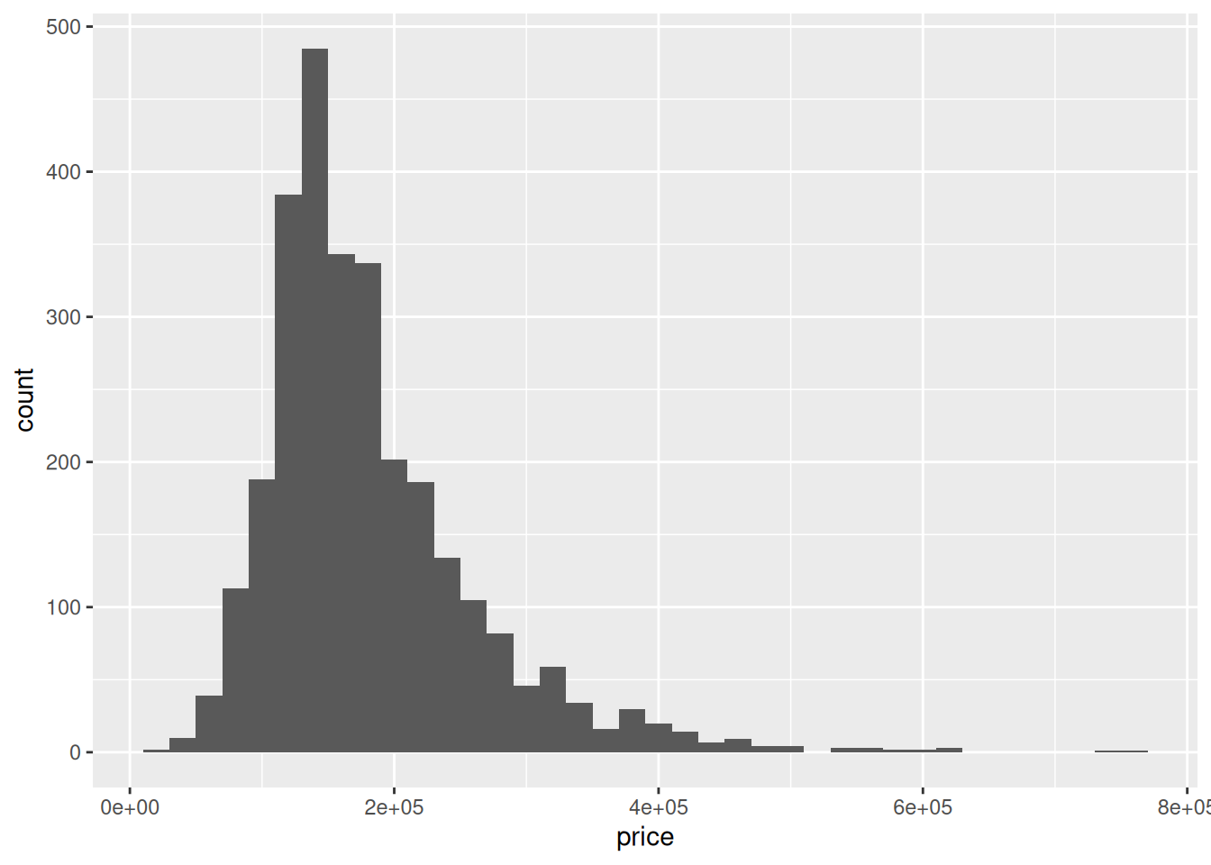

Price vs. square footage

How can we use square footage to model/predict pricing? Here is the model:

price_sqft_fit <- linear_reg() |>
  fit(price ~ sqft, data = housing)

tidy(price_sqft_fit)

# A tibble: 2 × 5
  term        estimate std.error statistic  p.value
  <chr>          <dbl>     <dbl>     <dbl>    <dbl>
1 (Intercept)   11430.   3271.        3.49 0.000482
2 sqft            114.      2.07     55.0  0       

And here is the model visualized:

ggplot(housing, aes(x = sqft, y = price)) +
  geom_point(alpha = 0.4) +
  geom_smooth(method = "lm")

`geom_smooth()` using formula = 'y ~ x'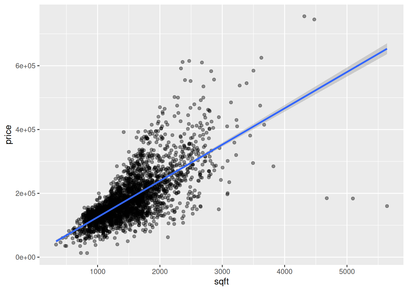

• Your turn: Write the equation of the model in mathematical notation. Then, interpret the intercept and slope.

\[ \widehat{price} = 11430.20 + 113.76 \times sqft \]

• Intercept: On average, we expect a home that is 0 square feet to cost $11430. This does not make sense in the context of the data - we won’t have a home that is 0 sq. ft.

• Slope: On average, for every 1 additional square foot, we expect hosue price to increase by $113.76

Price vs. home type

price_type_fit <- linear_reg() |>
  fit(price ~ home_type, data = housing)

tidy(price_type_fit)

# A tibble: 3 × 5
  term               estimate std.error statistic  p.value
  <chr>                 <dbl>     <dbl>     <dbl>    <dbl>
1 (Intercept)         185469.     1537.    121.   0       
2 home_typeDuplex     -45661.     7746.     -5.89 4.20e- 9
3 home_typeTownhouse  -49535.     8036.     -6.16 8.06e-10

• Your turn: Write the equation of the model in mathematical notation. Then, interpret the intercept and each coefficient in context.

\[ \widehat{price} = 185469.48 - 45660.54 \times Duplex - 49535.42 \times Townhouse \]

• Intercept: On average, we expect houses to cost 185469.48.

• Slope for Duplex: On average, we expect duplexes to cost 45660 dollars less than a house.

Price vs. square footage and home type

Now, let’s make some model that use both variables!

Main effects model

The main effects model is another name for the additive model. We fit the models below and wrote the model in math notation.

price_main_fit <- linear_reg() |>
  fit(price ~ sqft + home_type, data = housing)

tidy(price_main_fit)

# A tibble: 4 × 5
  term               estimate std.error statistic  p.value
  <chr>                 <dbl>     <dbl>     <dbl>    <dbl>
1 (Intercept)          13395.   3225.        4.15 3.38e- 5
2 sqft                   115.      2.03     56.5  0       
3 home_typeDuplex     -63251.   5338.      -11.8  1.19e-31
4 home_typeTownhouse  -20306.   5552.       -3.66 2.60e- 4

\[ \widehat{price} = 13394.8 + 114.5 \times sqft - 20306 \times Townhouse - 63251 \times Duplex \]

Task: Write the model equations for each home type. Provide interpretations of the coefficients.

House: $ = 13394.8 + 114.5 sqft $

• Intercept: On average, we expect a house with 0 square feet to cost $13394.8.
• Slope: On average, for houses, we expect every one additional square foot to correspond to an additional price of $114.5.

Townhouse: $ = (13394.8 - 20306) + 114.5 sqft $

• Intercept: On average, we expect a townhouse with 0 square feet to cost $-6911.2. This does not make sense in the context of the data - townhouses cannot be 0 sqft and prices cannot be negative.
• Slope: On average, for townhouses, we expect every one additional square foot to correspond to an additional price of $114.5.

Duplex: $ = (13394.8 - 63251) + 114.5 sqft $

• Intercept: On average, we expect a house with 0 square feet to cost -$49856.2. 49856.2. This does not make sense in the context of the data - duplexes cannot be 0 sqft and prices cannot be negative.
• Slope: On average, for duplexes, we expect every one additional square foot to correspond to an additional price of $114.5.

NOTE: Slopes are the SAME for all types!!

Interaction effects model

Now, we will fit an interaction effects model.

Task: Write code to fit an interaction effects model predicting price from square feet and home type.

price_inter_fit <- linear_reg() |>
  fit(price ~ sqft  * home_type, data = housing)

tidy(price_inter_fit)

# A tibble: 6 × 5
  term                    estimate std.error statistic  p.value
  <chr>                      <dbl>     <dbl>     <dbl>    <dbl>
1 (Intercept)               9087.    3273.       2.78  5.53e- 3
2 sqft                       117.       2.06    56.9   0       
3 home_typeDuplex          57547.   19114.       3.01  2.63e- 3
4 home_typeTownhouse       13970.   21910.       0.638 5.24e- 1
5 sqft:home_typeDuplex       -73.2     11.1     -6.58  5.56e-11
6 sqft:home_typeTownhouse    -26.9     17.0     -1.59  1.13e- 1

Task: Write the model output using mathematical notation.

\[ \widehat{price} = 9087 + 117 \times sqft + 139970 \times Townhouse + 57547 \times Duplex - 73 \times sqft \times Duplex - 27 \times sqft \times Townhouse \]

Task: Write the model equations for each home type.

House: $ = 9087 + 117 sqft $

Townhouse: $ = (9087 + 139970) + (117 - 27) sqft $

Duplex: $ = (9087 + 57547) + (117 - 73) sqft $

Model Comparison

So, we fit multiple models - how do we know which one is better?

We will dive into this tomorrow, but there is a value called adjusted \(R^2\) that lets us compare models. Higher values are better, lower are worse. You can glance() at a model fit to see the adjusted \(R^2\) values.

Which model is the best fit? Which is the worst?

glance(price_main_fit)

# A tibble: 1 × 12
  r.squared adj.r.squared  sigma statistic p.value    df  logLik    AIC    BIC
      <dbl>         <dbl>  <dbl>     <dbl>   <dbl> <dbl>   <dbl>  <dbl>  <dbl>
1     0.538         0.538 54532.     1112.       0     3 -35347. 70705. 70735.
# ℹ 3 more variables: deviance <dbl>, df.residual <int>, nobs <int>

glance(price_inter_fit)

# A tibble: 1 × 12
  r.squared adj.r.squared  sigma statistic p.value    df  logLik    AIC    BIC
      <dbl>         <dbl>  <dbl>     <dbl>   <dbl> <dbl>   <dbl>  <dbl>  <dbl>
1     0.545         0.545 54124.      687.       0     5 -35325. 70664. 70706.
# ℹ 3 more variables: deviance <dbl>, df.residual <int>, nobs <int>

Adjusted R squared is a higher for the interaction effects model - this is the better model! # One more model?

Task: Try adding one more variable to your chosen model from above. Does it make a difference in adjusted \(R^2\)?

price_inter_bed_fit <- linear_reg() |>
  fit(price ~ sqft  * home_type + bedrooms, data = housing)

glance(price_inter_bed_fit)

# A tibble: 1 × 12
  r.squared adj.r.squared  sigma statistic p.value    df  logLik    AIC    BIC
      <dbl>         <dbl>  <dbl>     <dbl>   <dbl> <dbl>   <dbl>  <dbl>  <dbl>
1     0.590         0.589 51421.      686.       0     6 -35178. 70371. 70419.
# ℹ 3 more variables: deviance <dbl>, df.residual <int>, nobs <int>

Adding the number of bedrooms greatly boosts the adjusted r squared value - this is a preferrable model!