Midterm + More Practice!

Lecture 10

May 29, 2025

Announcements

• I will not hold office hours on Tuesday, June 3rd: this is when you have your take home!
• Replacement midterm review office hours: June 2nd (3:30 - 5:30)
• Be in class and lab on Monday!!!!
• Tomorrow: Review game!

Midterm Exam 1

Worth 20% of your final grade; consists of two parts:

• In-class: worth 70% of the Midterm 1 grade;

• Take-home: worth 30% of the Midterm 1 grade.

Material

Everything we have done so far:

• plotting data with ggplot and interpreting plots
• computing and understanding summary statistics
• transforming data (row/column/grouping operations)
• pivoting & joining data
• data types/classes
• importing data
• Monday’s class: data science ethics

In-class

• All multiple choice

• You get both sides of one 8.5” x 11” note sheet that you and only you created (written, typed, iPad, etc)

Important

If you have testing accommodations, make sure I get proper documentation from SDAO and make appointments in the Testing Center ASAP. The appointment should overlap substantially with our class time if possible.

What should I put on my cheat sheet?

• description of common functions;
• examples of function usage;
• description of different visualizations: how to interpret, and what to use when;
• doodles;
• cute words of affirmation.

Warning

Don’t waste space on the details of any specific applications or datasets we’ve seen (penguins, Bechdel, gerrymandering, midwest, etc). Anything we want you to know about a particular application will be introduced from scratch within the exam.

Example in-class question

Which command can replace a pre-existing column in a data frame with a new and improved version of itself?

1. group_by
2. summarize
3. pivot_wider
4. geom_replace
5. mutate

Example in-class question

df

# A tibble: 6 × 2
      x y    
  <dbl> <chr>
1     1 Marie
2     2 Marie
3     3 Katie
4     4 Mary 
5     5 Mary 
6     6 Mary 

df |>
  group_by(y) |>
  summarize(xbar = mean(x))

How many rows will this output have?

1. 1
2. 2
3. 3
4. 6
5. 11

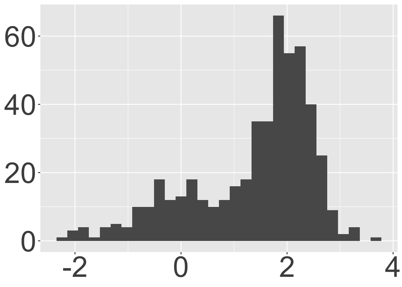
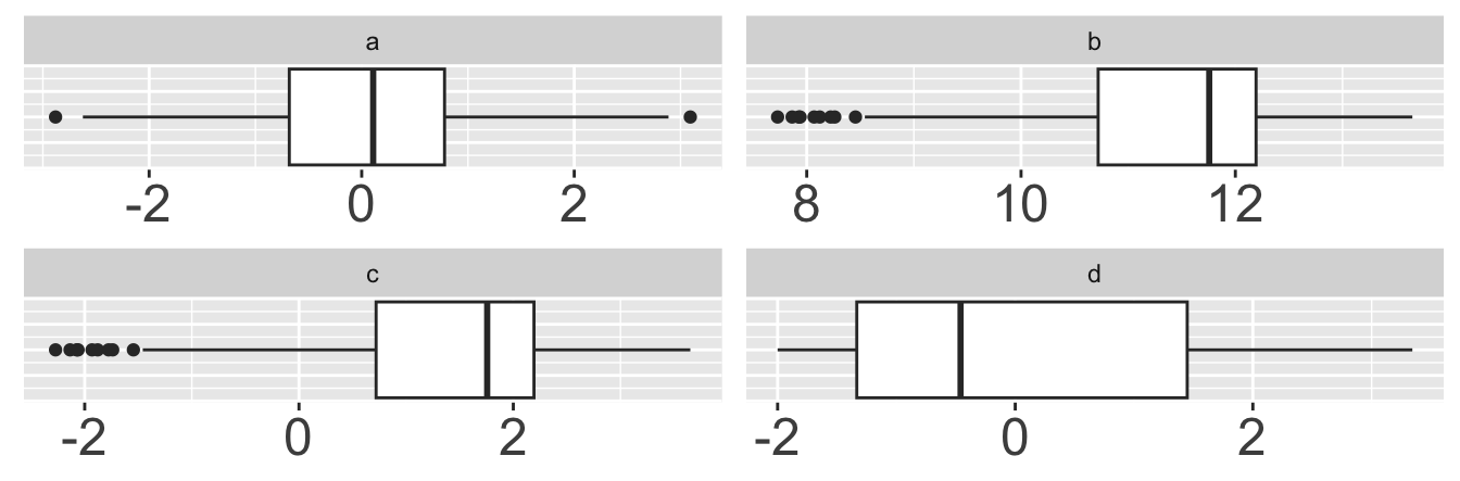
Example in-class question

Which box plot is visualizing the same data as the histogram?

Example in-class question

What code could have been used to produce df_result? Select all that apply.

df_X

state	year
LA	2025
NC	2025
LA	2024

df_Y

state	region
LA	south
NC	south
CA	west

df_result

state	year	region
LA	2025	south
NC	2025	south
LA	2024	south

1. left_join(df_X, df_Y)
   
2. right_join(df_X, df_Y)
   
3. full_join(df_X, df_Y)
   

4. anti_join(df_Y, df_X)
   
5. right_join(df_Y, df_X)
   

Take-home

• It will be just like a lab, but shorter;
• Completely open-resource, but citation policies apply;
• Absolutely no collaboration of any kind;
• Seek help by posting privately on Ed;
• Submit your final PDF to Gradescope in the usual way.

Reminder: conduct policies

• Uncited use of outside resources or inappropriate collaboration will result in a zero and be referred to the conduct office;
• If a conduct violation of any kind is discovered, your final letter grade in the course will be permanently reduced (A- down to B+, B+ down to B, etc);
• If folks share solutions, all students involved will be penalized equally, the sharer the same as the recipient.

Things you can do to study

• Practice problems: released Thursday February 13;
• Attend class tomorrow: review game
• Old labs: correct parts where you lost points;
• Old AEs: complete tasks we didn’t get to and compare with key;
• Code along: watch these videos specifically;
• Textbook: odd-numbered exercises in the back of IMS Chs. 1, 4, 5, 6

Let’s Practice!

Today’s Goals:

• Goal 1: Practice data transformation and working with characters - sales data from yesterday
• Goal 2: ✨Beautify✨ the plot from AE-08: plotting + factors
• Goal 3: Practice pivoting with AE-08 data

Goal 1: Transform Sales Data

Yesterday: read an Excel file with non-tidy data

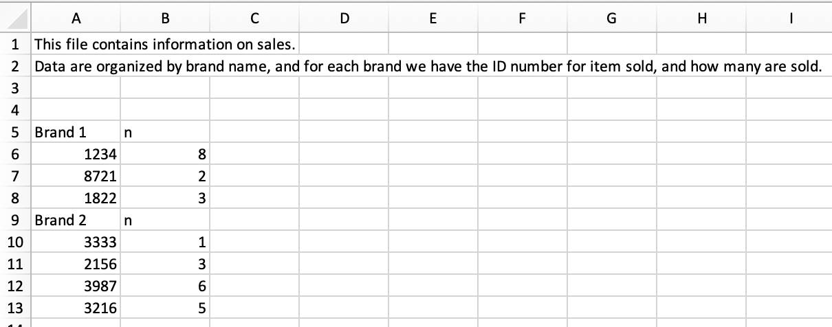
Goal 1: Transform Sales Data

Yesterday: read an Excel file with non-tidy data

Goal 1: Transform Sales Data

Goal: tidy up the data

String Functions

We’ve seen lots of functions that deal with numeric data (mean, median, sum, etc.) - what about characters?

• stringr is a tidyverse package with lots of functions for dealing with character strings

• today: str_detect in stringr

String Functions

• str_detect() identifies if some characters are a substring of a larger string

• useful in cases when you need to check some condition, for example:

  • in a filter()

  • in an if_else() or case_when()

String Functions

• str_detect() identifies if some characters are a substring of a larger string

• useful in cases when you need to check some condition, for example:

  • in a filter()

  • in an if_else() or case_when()

example: which classes in a list are in the stats department?

classes <- c("sta199", "dance122", "math185", "sta240", "pubpol202")
str_detect(classes, "sta")

[1]  TRUE FALSE FALSE  TRUE FALSE

String Functions

General form:

str_detect(character_var, "word_to_detect")

Let’s get started!

Open up yesterday’s AE file (AE-09).

Let’s get started!

sales_raw <- read_excel(
  "data/sales.xlsx", 
  skip = 3,
  col_names = c("id", "n")
  )

# A tibble: 9 × 2
  id      n    
  <chr>   <chr>
1 Brand 1 n    
2 1234    8    
3 8721    2    
4 1822    3    
5 Brand 2 n    
6 3333    1    
7 2156    3    
8 3987    6    
9 3216    5    

Create Brand Column

sales_raw 

# A tibble: 9 × 2
  id      n    
  <chr>   <chr>
1 Brand 1 n    
2 1234    8    
3 8721    2    
4 1822    3    
5 Brand 2 n    
6 3333    1    
7 2156    3    
8 3987    6    
9 3216    5    

Create Brand Column

sales_raw |>
  mutate(
    is_brand_name = str_detect(id, "Brand")
  )

# A tibble: 9 × 3
  id      n     is_brand_name
  <chr>   <chr> <lgl>        
1 Brand 1 n     TRUE         
2 1234    8     FALSE        
3 8721    2     FALSE        
4 1822    3     FALSE        
5 Brand 2 n     TRUE         
6 3333    1     FALSE        
7 2156    3     FALSE        
8 3987    6     FALSE        
9 3216    5     FALSE        

Create Brand Column

sales_raw |>
  mutate(
    is_brand_name = str_detect(id, "Brand"),
    brand = if_else(is_brand_name, id, NA)
  )

# A tibble: 9 × 4
  id      n     is_brand_name brand  
  <chr>   <chr> <lgl>         <chr>  
1 Brand 1 n     TRUE          Brand 1
2 1234    8     FALSE         <NA>   
3 8721    2     FALSE         <NA>   
4 1822    3     FALSE         <NA>   
5 Brand 2 n     TRUE          Brand 2
6 3333    1     FALSE         <NA>   
7 2156    3     FALSE         <NA>   
8 3987    6     FALSE         <NA>   
9 3216    5     FALSE         <NA>   

Create Brand Column

sales_raw |>
  mutate(
    is_brand_name = str_detect(id, "Brand"),
    brand = if_else(is_brand_name, id, NA)
  )|>
  fill(brand)

# A tibble: 9 × 4
  id      n     is_brand_name brand  
  <chr>   <chr> <lgl>         <chr>  
1 Brand 1 n     TRUE          Brand 1
2 1234    8     FALSE         Brand 1
3 8721    2     FALSE         Brand 1
4 1822    3     FALSE         Brand 1
5 Brand 2 n     TRUE          Brand 2
6 3333    1     FALSE         Brand 2
7 2156    3     FALSE         Brand 2
8 3987    6     FALSE         Brand 2
9 3216    5     FALSE         Brand 2

Keep Needed Rows

sales_raw |>
  mutate(
    is_brand_name = str_detect(id, "Brand"),
    brand = if_else(is_brand_name, id, NA)
  )|>
  fill(brand)|>
  filter(!is_brand_name)

# A tibble: 7 × 4
  id    n     is_brand_name brand  
  <chr> <chr> <lgl>         <chr>  
1 1234  8     FALSE         Brand 1
2 8721  2     FALSE         Brand 1
3 1822  3     FALSE         Brand 1
4 3333  1     FALSE         Brand 2
5 2156  3     FALSE         Brand 2
6 3987  6     FALSE         Brand 2
7 3216  5     FALSE         Brand 2

Keep Needed Columns

sales_raw |>
  mutate(
    is_brand_name = str_detect(id, "Brand"),
    brand = if_else(is_brand_name, id, NA)
  )|>
  fill(brand)|>
  filter(!is_brand_name)|>
  select(brand, id, n)

# A tibble: 7 × 3
  brand   id    n    
  <chr>   <chr> <chr>
1 Brand 1 1234  8    
2 Brand 1 8721  2    
3 Brand 1 1822  3    
4 Brand 2 3333  1    
5 Brand 2 2156  3    
6 Brand 2 3987  6    
7 Brand 2 3216  5    

Goal 2: Beautify AE-08 Plot

Data:

durham_climate 

# A tibble: 12 × 4
   month     avg_high_f avg_low_f precip
   <chr>          <dbl>     <dbl>  <dbl>
 1 January           49        28   4.45
 2 February          53        29   3.7 
 3 March             62        37   4.69
 4 April             71        46   3.43
 5 May               79        56   4.61
 6 June              85        65   4.02
 7 July              89        70   3.94
 8 August            87        68   4.37
 9 September         81        60   4.37
10 October           71        47   3.7 
11 November          62        37   3.39
12 December          53        30   3.43

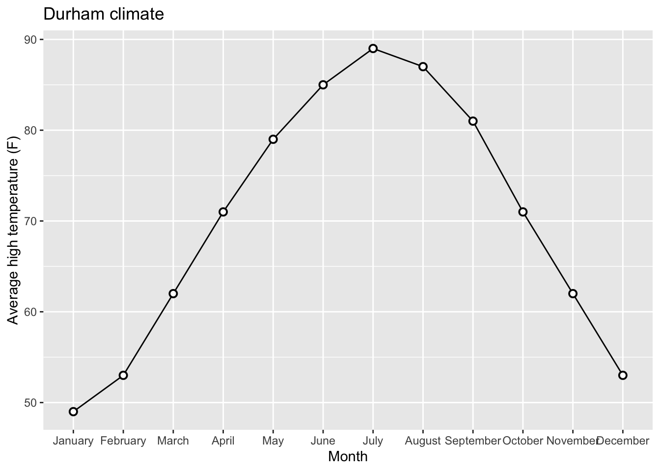
Goal 2: Beautify AE-08 Plot

Original Plot:

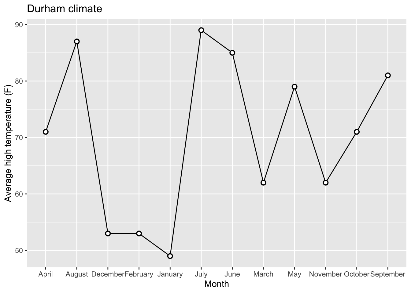
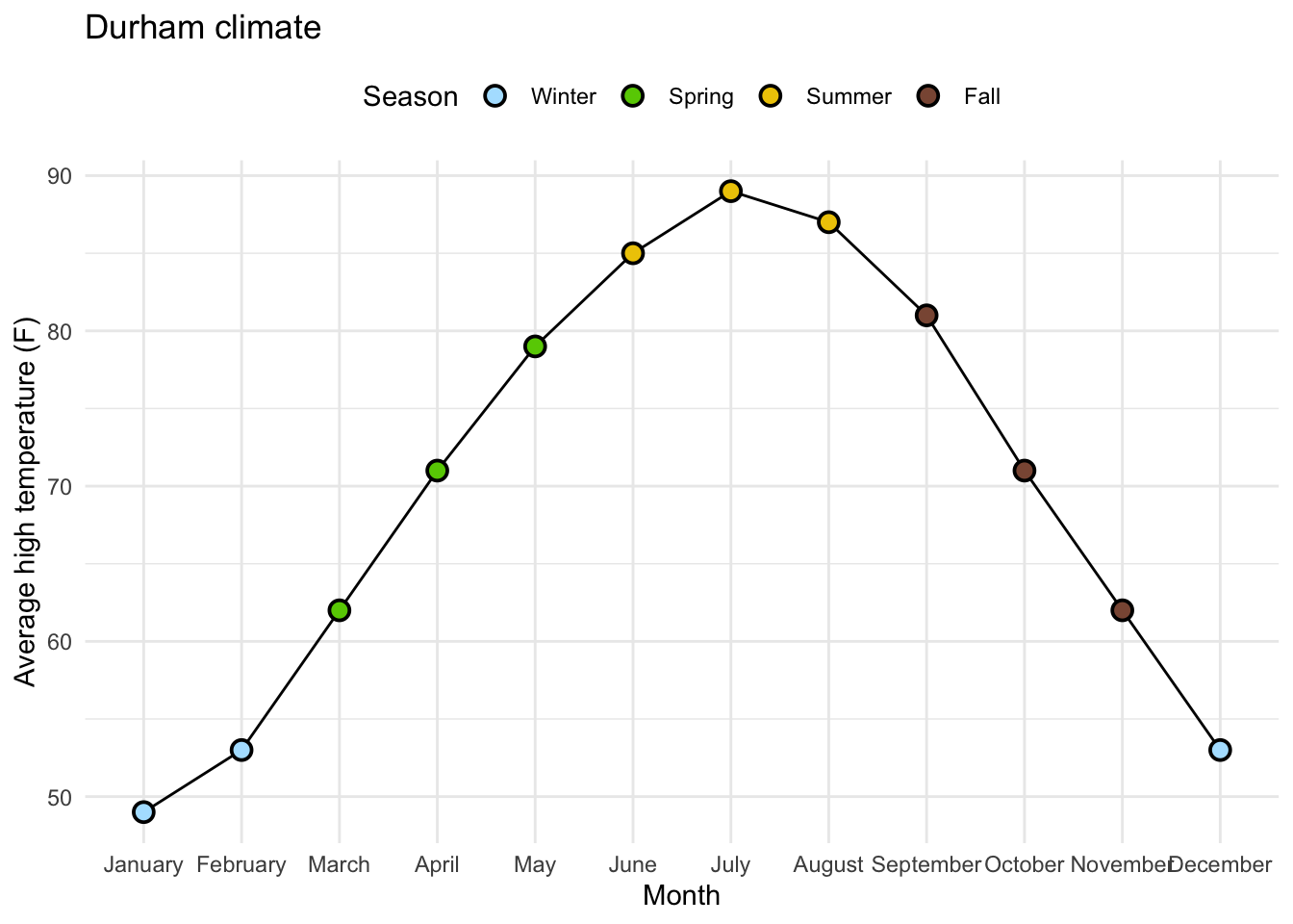
Goal 2: Beautify AE-08 Plot

Releveling Months:

Goal 2: Beautify AE-08 Plot

Goal:

Goal: Beautify AE-08 Plot

# A tibble: 12 × 4
   month     avg_high_f avg_low_f precip
   <fct>          <dbl>     <dbl>  <dbl>
 1 January           49        28   4.45
 2 February          53        29   3.7 
 3 March             62        37   4.69
 4 April             71        46   3.43
 5 May               79        56   4.61
 6 June              85        65   4.02
 7 July              89        70   3.94
 8 August            87        68   4.37
 9 September         81        60   4.37
10 October           71        47   3.7 
11 November          62        37   3.39
12 December          53        30   3.43

The Code…

Take a look at the printout!W hat does each highlighted portion do?

The Code…

Go ahead and pull today’s AE - mess around with the code.

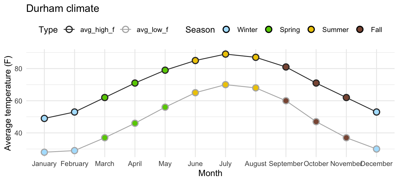
Goal 3: High/Low lines

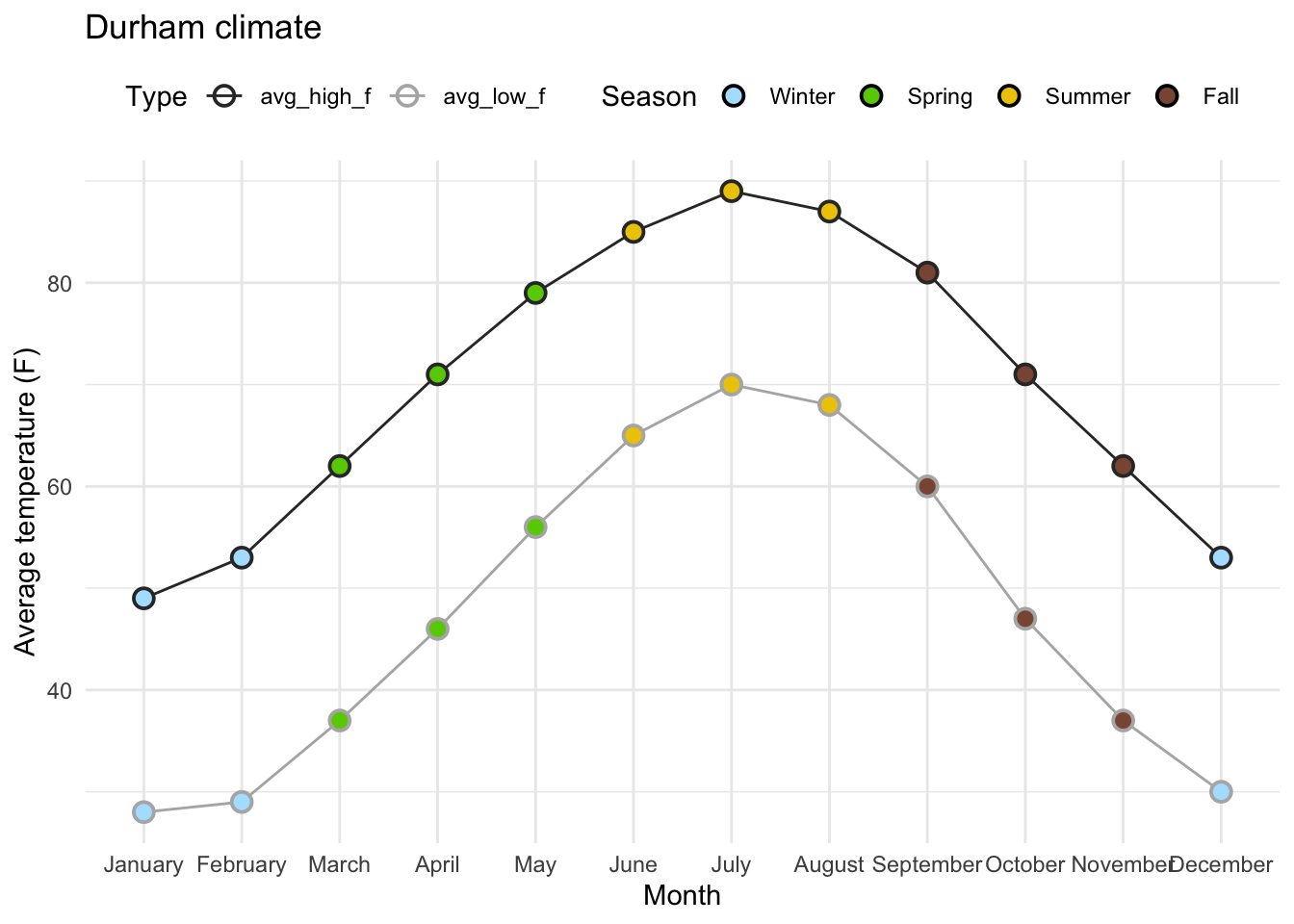
Goal 3: High/Low lines

# A tibble: 3 × 5
  month    avg_high_f avg_low_f precip season
  <fct>         <dbl>     <dbl>  <dbl> <fct> 
1 January          49        28   4.45 Winter
2 February         53        29   3.7  Winter
3 March            62        37   4.69 Spring

Pivot!!!

# A tibble: 5 × 5
  month    avg_high_f avg_low_f precip season
  <fct>         <dbl>     <dbl>  <dbl> <fct> 
1 January          49        28   4.45 Winter
2 February         53        29   3.7  Winter
3 March            62        37   4.69 Spring
4 April            71        46   3.43 Spring
5 May              79        56   4.61 Spring

# A tibble: 5 × 5
  month    precip season temp_type   temp
  <fct>     <dbl> <fct>  <chr>      <dbl>
1 January    4.45 Winter avg_high_f    49
2 January    4.45 Winter avg_low_f     28
3 February   3.7  Winter avg_high_f    53
4 February   3.7  Winter avg_low_f     29
5 March      4.69 Spring avg_high_f    62

Pivot!!!

Add your pivot code to today’s AE. Check out the plotting code! What is going on?