── Attaching core tidyverse packages ────────────── tidyverse 2.0.0 ──
✔ dplyr     1.1.4     ✔ readr     2.1.5
✔ forcats   1.0.0     ✔ stringr   1.5.1
✔ ggplot2   3.5.1     ✔ tibble    3.2.1
✔ lubridate 1.9.3     ✔ tidyr     1.3.1
✔ purrr     1.0.2
── Conflicts ──────────────────────────────── tidyverse_conflicts() ──
✖ dplyr::filter() masks stats::filter()
✖ dplyr::lag()    masks stats::lag()
ℹ Use the conflicted package (<http://conflicted.r-lib.org/>) to force all conflicts to become errors
library(palmerpenguins)
library(ggthemes)
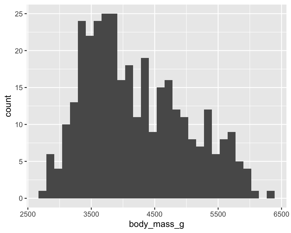
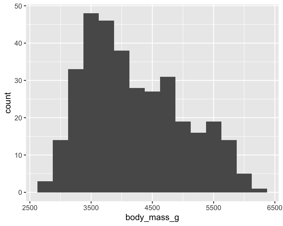
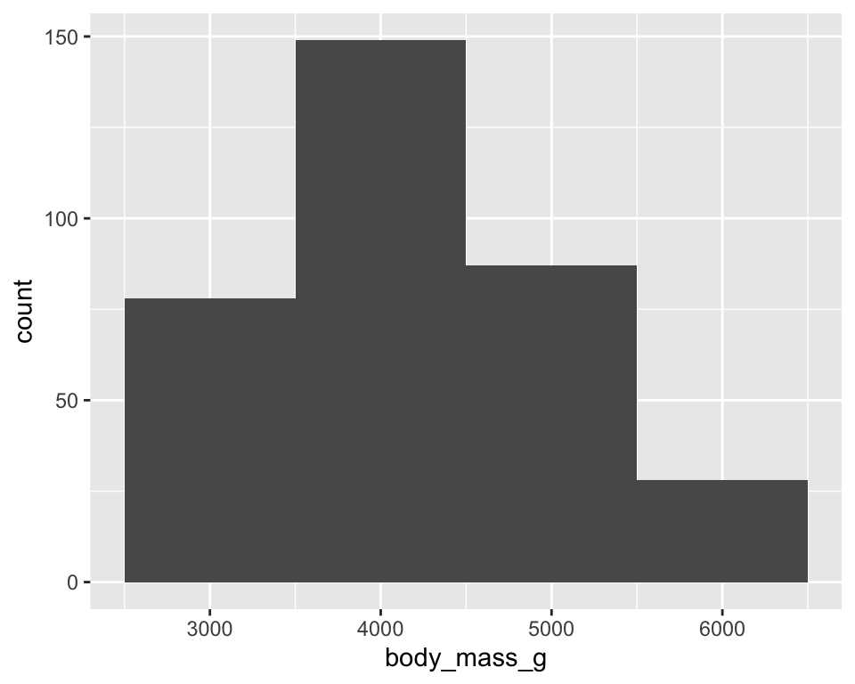
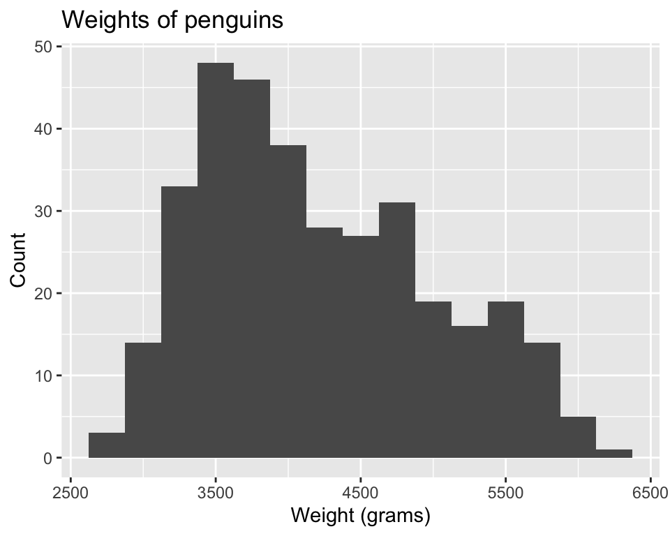
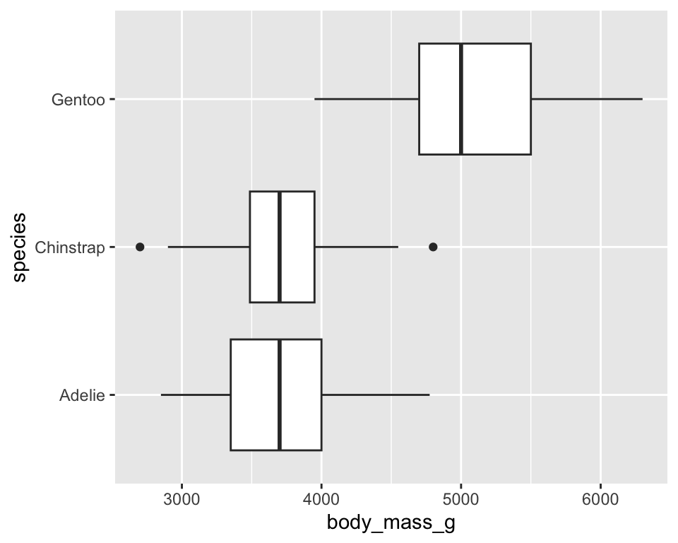
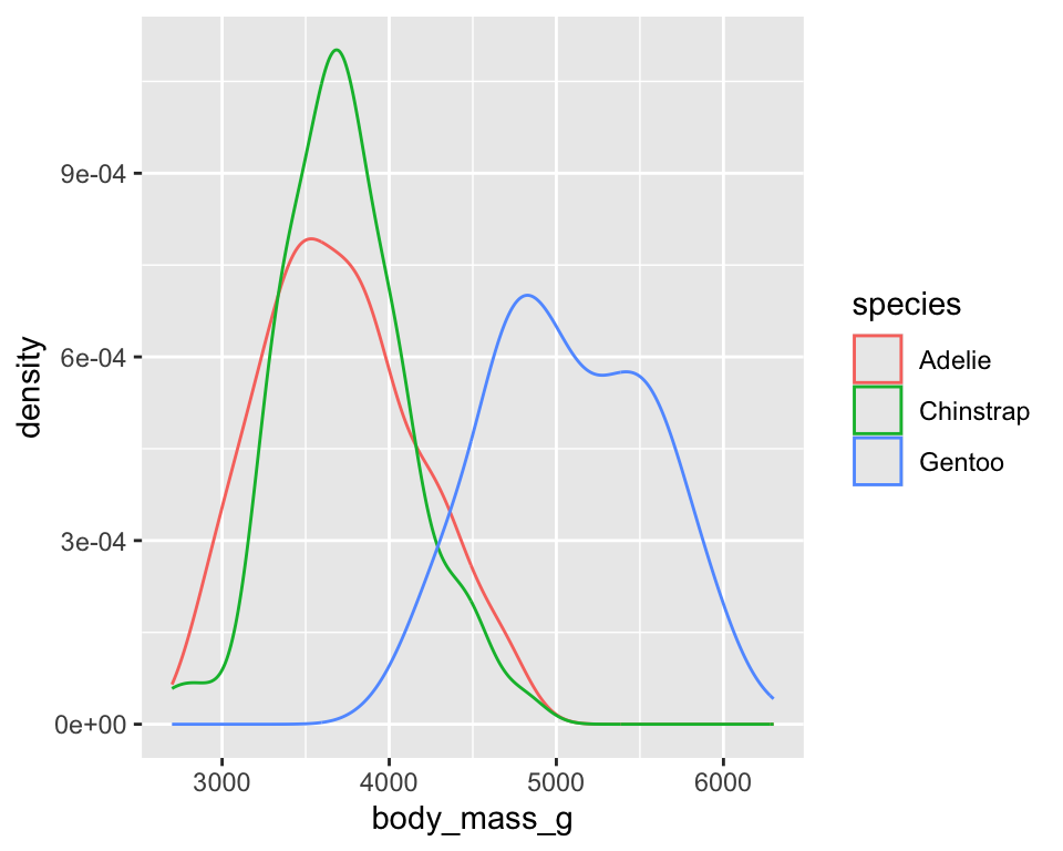
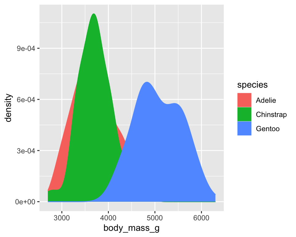
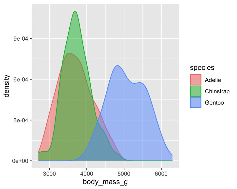
penguins
# A tibble: 344 × 8
   species island    bill_length_mm bill_depth_mm flipper_length_mm
   <fct>   <fct>              <dbl>         <dbl>             <int>
 1 Adelie  Torgersen           39.1          18.7               181
 2 Adelie  Torgersen           39.5          17.4               186
 3 Adelie  Torgersen           40.3          18                 195
 4 Adelie  Torgersen           NA            NA                  NA
 5 Adelie  Torgersen           36.7          19.3               193
 6 Adelie  Torgersen           39.3          20.6               190
 7 Adelie  Torgersen           38.9          17.8               181
 8 Adelie  Torgersen           39.2          19.6               195
 9 Adelie  Torgersen           34.1          18.1               193
10 Adelie  Torgersen           42            20.2               190
# ℹ 334 more rows
# ℹ 3 more variables: body_mass_g <int>, sex <fct>, year <int>